
Exponential Growth vs. Decay: Quick Warm Up
Loading the math board and drawing, please wait…
In collections
Exponential & Logarithmic Functions
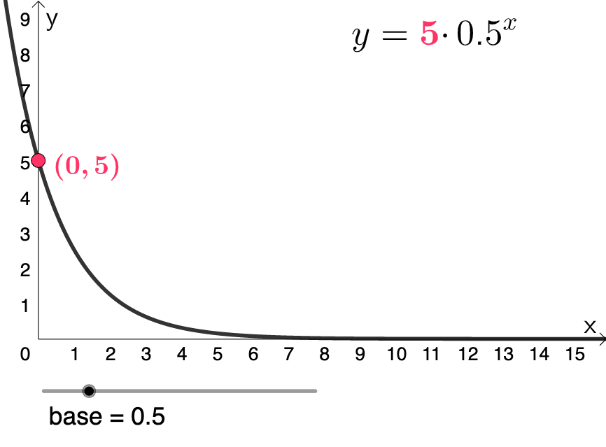
This example demonstrates the comparison of exponential growth and decay functions. It involves core math concepts like exponential functions, growth rates, decay rates, and function graphs. Constructed using GeoGebra commands base, b, A, f, text1 to model the functions and show parameter variations. Suitable for high school mathematics teaching to understand the properties of exponential functions and their real-world applications.
GeoGebra Commands & Parameters
Numeric base(0.5)Numeric b(5)(0, b)f(x) = (b * base^(x))
AI Drawing Prompt Reference
In a single coordinate plane, draw exponential function graphs to compare exponential growth and decay behavior. Set the base to 0.5 and choose the parameter b as 5, then include the point (0, b) on the graph. Define the function f(x) = b · base^x and plot its curve, so the relationship between the base, the parameter b, and how the function changes with x is clearly reflected.
The prompt above was compiled from the original drawing commands and is for reference only.