
Exponential Growth & Decay Visualization
Loading the math board and drawing, please wait…
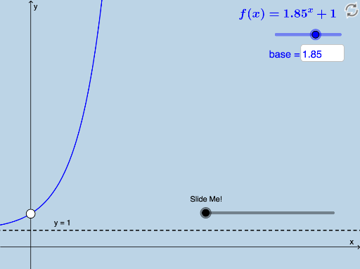
This example dynamically illustrates exponential growth and decay. Key mathematical concepts include exponential functions and their graph characteristics. Using GeoGebra commands like Vector, Translate, Polygon, and Dilate, the impact of parameter changes on the function graph can be observed intuitively. Suitable for high school mathematics education, particularly in exponential functions and calculus courses.
GeoGebra Commands & Parameters
Vector((0, 0), (1, 0)) → uTranslate(G, u) → G'Translate(B, u) → B'Translate(C, u) → C'Translate(D, u) → D'Translate(A, u) → A'Polygon(A, A', B) → poly1, b, a_1, a'Polygon(B, B', C) → poly2, c, b_1, b'Polygon(C, C', D) → poly3, d, c_1, c'Polygon(D, D', E) → poly4, e, d_1, d'Dilate(A, If[0 < o ≤ 1, 1 - o, 0], A') → A'_1Dilate(B, If[0 < o ≤ 1, 1 - o, 0], B') → B'_1Dilate(C, If[0 < o ≤ 1, 1 - o, 0], C') → C'_1Dilate(D, If[0 < o ≤ 1, 1 - o, 0], D') → D'_1Segment(A, A'_1) → pSegment(B, B'_1) → qSegment(C, C'_1) → rSegment(D, D'_1) → sDilate(A'_1, If[1 < o ≤ 2, 2 - o, 0], B) → HSegment(A'_1, H) → tDilate(A'_1, If[2 < o ≤ 3, 3 - o, 0], B'_1) → IVector(A'_1, I) → vTranslate(A'_1, v) → JTranslate(H, v) → H'Segment(J, H') → t'Dilate(B'_1, If[3 < o ≤ 4, 4 - o, 0], C'_1) → KVector(B'_1, K) → wTranslate(J, w) → J'Translate(H', w) → H''Segment(J', H'') → t''Dilate(C'_1, If[4 < o ≤ 5, 5 - o, 0], D'_1) → MVector(C'_1, M) → u_1Translate(J', u_1) → J''Translate(H'', u_1) → H'''Segment(J'', H''') → t'''Translate(L, u) → L'Translate(F, u) → F'Line(A, B) → f_1IntegralBetween(f, g, 0, 1) → e_1Translate(O, u) → O'IntegralBetween(f, g_1, 1, 2) → h_1IntegralBetween(f, h, 2, 3) → i_1Dilate(O, If[0 < p_1 ≤ 1, 1 - p_1, 0], O') → O'_1Dilate(L, If[0 < p_1 ≤ 1, 1 - p_1, 0], L') → L'_1Dilate(G, If[0 < p_1 ≤ 1, 1 - p_1, 0], G') → G'_1Segment(O, O'_1) → l_1Segment(L, L'_1) → m_1Dilate(G'_1, If[1 < p_1 ≤ 2, 2 - p_1, 0], O) → PSegment(G'_1, P) → q_1Dilate(G'_1, If[2 < p_1 ≤ 3, 3 - p_1, 0], O'_1) → SVector(G'_1, S) → v_1Translate(G'_1, v_1) → TTranslate(P, v_1) → P'Segment(O'_1, L) → r_1Dilate(O'_1, If[4 < p_1 ≤ 5, 5 - p_1, 0], L'_1) → WVector(O'_1, W) → s_1Translate(O'_1, s_1) → ZTranslate(L, s_1) → L'_2Translate(G, u) → G'_2Translate(C_1, u) → F_1Translate(D_1, u) → G_1Dilate(G, If[0 < a_2 ≤ 1, 1 - a_2, 0], G'_2) → G'_3Dilate(C_1, If[0 < a_2 ≤ 1, 1 - a_2, 0], F_1) → H_1Dilate(D_1, If[0 < a_2 ≤ 1, 1 - a_2, 0], G_1) → I_1Segment(G, G'_3) → g_2Segment(C_1, H_1) → h_2Segment(D_1, I_1) → i_2Dilate(G'_2, If[1 < a_2 ≤ 2, 2 - a_2, 0], C_1) → J_1Segment(G'_2, J_1) → j_2IntegralBetween(f, g, 0, 1) → b_2IntegralBetween(f, g_1, 1, 2) → c_2IntegralBetween(f, h, 2, 3) → d_2Segment(D_1, F_1) → k_2Circle(F_1, e_2) → p_2Intersect(p_2, k_2) → K_1,Circle(K_1, e_2) → q_2Intersect(q_2, k_2) → L_1, M_1Dilate(G'_2, If[2 < a_2 ≤ 3, 3 - a_2, 0], M_1) → N_1Vector(G'_2, N_1) → v_2Translate(G'_2, v_2) → O_1Translate(J_1, v_2) → P_1Segment(O_1, P_1) → l_2Rotate(O_1, If[3 < a_2 ≤ 4, ((a_2 - 3) * π), π], K_1) → R_1Rotate(P_1, If[3 < a_2 ≤ 4, ((a_2 - 3) * π), π], K_1) → S_1Segment(R_1, S_1) → m_2Rotate(R_1, If[4 < a_2 ≤ 5, ((a_2 - 4) * π), π], L_1) → T_1Rotate(S_1, If[4 < a_2 ≤ 5, ((a_2 - 4) * π), π], L_1) → U_1Segment(T_1, U_1) → n_2Segment(M_1, D_1) → r_2Dilate(M_1, If[5 < a_2 ≤ 6, 6 - a_2, 0], G_1) → Q_1Vector(M_1, Q_1) → w_2Translate(M_1, w_2) → V_1Translate(D_1, w_2) → W_1Segment(V_1, W_1) → s_2Midpoint(W_1, E_1) → Z_1Rotate(V_1, If[6 < a_2 ≤ 7, ((a_2 - 6) * π), π], W_1) → A_2Rotate(W_1, If[6 < a_2 ≤ 7, ((a_2 - 6) * π), π], W_1) → B_2Segment(A_2, B_2) → t_2Rotate(A_2, If[7 < a_2 ≤ 8, ((a_2 - 7) * π), π], Z_1) → C_2Rotate(B_2, If[7 < a_2 ≤ 8, ((a_2 - 7) * π), π], Z_1) → D_2Segment(C_2, D_2) → f_3Translate(F, u) → F'_1Intersect(f, n, (4, 12.713506250000002)) → E_2Dilate(F, If[0 < p_1 ≤ 1, 1 - p_1, 0], F'_1) → F'_2Segment(F, F'_2) → g_3Dilate(O'_1, If[2 < p_1 ≤ 3, 3 - p_1, 0], L) → QSegment(O'_1, Q) → j_1Distance(O'_1, L) → distanceO'1LDilate(L'_1, If[3 < p_1 ≤ 4, 4 - p_1, 0], F) → RSegment(L'_1, R) → t_1Distance(L'_1, F) → distanceL'1FDilate(F'_1, If[4 < p_1 ≤ 5, 5 - p_1, 0], N) → USegment(F'_1, U) → f_2IntegralBetween(f, k_1, x(F), x(F'_1)) → w_1Distance(F'_1, N) → distanceF'1NTextfield(base) → InputBox1Segment(G, G'_1) → i_3
AI Drawing Prompt Reference
Create a dynamic visualization of exponential growth and decay, featuring multiple polygons and lines. Start by drawing a horizontal vector, then translate four points based on this vector to get four new points. Form four adjacent polygons using these eight points, observing how parameter changes affect their shapes. Next, scale each polygon and connect the scaled vertices to the original vertices with lines. Finally, draw several lines connecting specific points and calculate the integral of a function over given intervals, representing the results with different colors or styles.
The prompt above was compiled from the original drawing commands and is for reference only.