
Exploring Pythagoras: Dynamic Geometry Demonstration
Loading the math board and drawing, please wait…
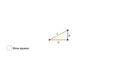
① This interactive GeoGebra example visually demonstrates the Pythagorean theorem by showing the relationship between the areas of squares constructed on the sides of a right triangle. ② Core mathematical concepts include right triangles, square areas, the sum of squares of legs equaling the square of the hypotenuse, and the cosine rule as a degenerate case for right angles. ③ Construction highlights: using GeoGebra commands such as Intersect, Point, Segment, OrthogonalLine, Polygon, Line, and Circle, the example builds a right triangle ABC and squares on each side (poly1, poly2, poly3), with auxiliary lines, circles, and parametric curves (e.g., a_{12}, b_{13}) to illustrate area relationships. Objects include points A, B, C, D, E, F, G, H, I, J, K, L, M; segments f, g, h, i, k, l, m, a, p, q, r, b, t, c_6, d, e, f_1, b_2, b_1, i_1; and polygons poly1, poly2, poly3, poly4. ④ Suitable for middle school to high school students learning geometry and algebra connections, and useful for teachers demonstrating or students exploring multiple proofs of the Pythagorean theorem.
GeoGebra Commands & Parameters
Intersect(xAxis, yAxis) → APoint(xAxis) → BSegment(A, B) → fOrthogonalLine(B, f) → gPoint(g) → CSegment(A, C) → hSegment(C, B) → iPolygon(A, C, 4) → poly1, c, k, l, m, D, EPolygon(C, B, 4) → poly2, a, p, q, r, F, GPolygon(B, A, 4) → poly3, b, t, a_{12}, b_{13}, H, ILine(A, F) → c_6Circle(F, 1) → dIntersect(d, c_6, 2) → JCircle(J, f) → eIntersect(e, c_6, 2) → KPolygon(K, J, 4) → poly4, f_1, b_2, b_1, i_1, L, MOrthogonalLine(K, c_6) → j_1Circle(K, i) → c_5Intersect(c_5, j_1, 2) → NPolygon(N, K, 4) → poly5, k_1, l_1, a_2, a_1, O, POrthogonalLine(E, c_6) → p_1Intersect(c_6, p_1) → QCircle(Q, 1) → d_1Intersect(d_1, c_6, 1) → RCircle(R, f) → e_1Intersect(e_1, c_6, 1) → SOrthogonalLine(R, c_6) → q_1Circle(R, i) → r_1Intersect(r_1, q_1, 2) → TPolygon(S, T, 4) → poly6, s_1, t_1, a_9, b_{10}, U, VOrthogonalLine(V, c_6) → f_2OrthogonalLine(U, q_1) → g_2Line(J, L) → h_2Line(N, P) → i_2Line(P, O) → j_2Line(M, L) → k_2Intersect(h_2, i_2) → WIntersect(j_2, k_2) → ZIntersect(f_2, g_2) → A_1Intersect(q_1, g_2) → B_1Intersect(c_6, f_2) → C_1Polygon(A_1, V, U) → t1, a_5, a_{10}, b_5Polygon(B_1, U, T) → t2, a_6, b_{11}, b_6Polygon(T, S, R) → t3, r_2, b_7, a_7Polygon(S, C_1, V) → t4, a_8, b_8, c_2Polygon(J, W, N) → t5, a_3, b_3, c_1Polygon(J, K, N) → t6, n_3, j_4, k_3Polygon(M, Z, K) → t7, a_4, m_2, z_1Polygon(Z, K, O) → t8, c_4, z_2, b_4Polygon(C, A, B) → t9, b_{12}, c_3, a_{11}
AI Drawing Prompt Reference
Draw a right triangle ABC, and construct three squares outside each side, labeled as poly1, poly2, and poly3. Use auxiliary lines and circles to demonstrate that the area of the square on the hypotenuse is equal to the sum of the areas of the squares on the legs. Add more auxiliary lines and circles to construct several smaller squares and polygons to further illustrate the area relationships.
The prompt above was compiled from the original drawing commands and is for reference only.