
Exploring Cubic Gradients
Loading the math board and drawing, please wait…
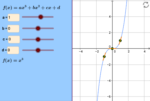
This example demonstrates the relationship between cubic functions and their derivatives, involving core math concepts like derivatives, function graphs, and rates of change. It is constructed using GeoGebra commands such as If, panelleft1, panelleft2, Textfield, Sequence, Derivative, with objects like a, f_3, b, f_2, c, f_1, etc. Suitable for high school and above students to understand the geometric meaning of derivatives in calculus and properties of cubic functions.
GeoGebra Commands & Parameters
If(a ≟ 1, x^(3), (a * x^(3))) → f_3If(b ≟ 1, x^(2), (b * x^(2))) → f_2If(c ≟ 1, x, (c * x)) → f_1panelleft1(240) → panel1, e, i, j, k, lpanelleft2(240) → panel2, m, n, p, q, rTextfield(a) → InputBox1Textfield(b) → InputBox2Textfield(c) → InputBox3Sequence((i, f(i)), i, -4, 4) → intpointsIf(b ≟ 0, If[c ≟ 0, f_3(x) + d, f_3(x) + f_1(x) + d], If[c ≟ 0, f_3(x) + f_2(x) + d, f_3(x) + f_2(x) + f_1(x) + d]) → gTextfield(d) → InputBox5Sequence(Segment[Intersect[Circle[(i, f(i)), 0.5], Line[(i, f(i)), (i + 1, f(i) + f'(i))], 1], Intersect[Circle[(i, f(i)), 0.5], Line[(i, f(i)), (i + 1, f(i) + f'(i))], 2]], i, -4, 4) → chordsSequence((i, f'(i)), i, -4, 4) → gradientsDerivative(f) → f'