
Function Mapping Diagram
Loading the math board and drawing, please wait…
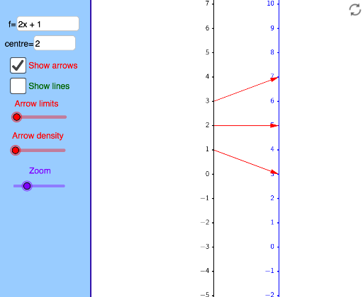
This example demonstrates how a function can be represented using a mapping diagram instead of a graph. It involves the concept of functions, particularly how mapping diagrams help understand the input-output relationship. GeoGebra commands used include TableText, Corner, Distance, Line, Text, panelleft1, Textfield, If, Sequence, Vector, Zip, etc. Suitable for high school math education to help students visually understand function properties.
GeoGebra Commands & Parameters
TableText({{"0"}, {"\ \ \ \ \ \ \ \ \ \ \ \ \ \ \ \ "}}, "hc") → Xt0Corner(1) → corner1Corner(2) → corner2Corner(3) → corner3Corner(4) → corner4Corner(5) → screenDimDistance(corner1, corner2) → distXDistance(corner1, corner4) → distYLine(OY, yAxis) → YaxisLineText("(x,y) = (" + (x(A)) + "," + (y(A)) + ") in black coordinate system") → text2Text("(X,Y) = (" + (x(A) - x(OY)) + "," + (y(A) - y(OY)) + ") in blue coordinate system") → text1panelleft1(panelsize) → panelquad, panelseg1, panelseg2, panelseg3, panelseg4, panellineTextfield(f) → InputBox1Line(OX, yAxis) → XaxisLineTextfield(x0) → InputBox2If(minstepfrac > lg(5), 10^(minsteppower + 1), If[minstepfrac > lg(2), (5 * 10^(minsteppower)), If[minstepfrac > 0, (2 * 10^(minsteppower)), 10^(minsteppower)]]) → stepsizeSequence(Text[TableText[{{"\phantom{(}" + (x0 + (n * stepsize)) + ""}, {"\phantom{(} \ \ \ \ \ \ \ \ \ \ \ \ \ \ \ "}}, "hr"], (x(OX) - Distance[Corner[Xt0, 1], Corner[Xt0, 2]] + 7 / unitX, (n * steplength) + y(OX) + (Distance[Corner[Xt0, 1], Corner[Xt0, 4]] * 0.25) + 4 / unitY), true, true], n, ceil((y(Corner[1]) - y(OX)) / steplength), floor((y(Corner[4]) - y(OX)) / steplength)) → XaxisNumbersSequence(Segment[(x(OX), y(OX) + (n * steplength)), (x(OX) - 2 / unitX, y(OX) + (n * steplength))], n, ceil((y(Corner[1]) - y(OX)) / steplength), floor((y(Corner[4]) - y(OX)) / steplength)) → XaxisTicksSequence(Text[TableText[{{"\phantom{(}" + (y0 + (n * stepsize)) + ""}, {"\phantom{(} \ \ \ \ \ \ \ \ \ \ \ \ \ \ \ "}}, "hr"], (x(OY) - Distance[Corner[Xt0, 1], Corner[Xt0, 2]] + 7 / unitX, (n * steplength) + y(OY) + (Distance[Corner[Xt0, 1], Corner[Xt0, 4]] * 0.25) + 4 / unitY), true, true], n, ceil((y(Corner[1]) - y(OY)) / steplength), floor((y(Corner[4]) - y(OY)) / steplength)) → YaxisNumbersSequence(Segment[(x(OY), y(OY) + (n * steplength)), (x(OY) - 2 / unitX, y(OY) + (n * steplength))], n, ceil((y(Corner[1]) - y(OY)) / steplength), floor((y(Corner[4]) - y(OY)) / steplength)) → YaxisTicksVector((xpos, 0), (ypos, 0)) → uSequence(i / spacing, i, ((-numarrows) * spacing), (numarrows * spacing)) → arrowstartsZip(x0 + (as * numminstep), as, arrowstarts) → arrowxvalsZip(f(ax), ax, arrowxvals) → arrowyvalsZip((xpos, ((xv - x0) * steplength / stepsize)), xv, arrowxvals) → arrowxcoordsZip((ypos, ((yv - y0) * steplength / stepsize)), yv, arrowyvals) → arrowycoordsZip(Vector[ax, ay], ax, arrowxcoords, ay, arrowycoords) → arrowsZip(Line[ax, ay], ax, arrowxcoords, ay, arrowycoords) → linesVector((xpos, 0), (ypos, 0)) → v
AI Drawing Prompt Reference
Draw a function mapping diagram to illustrate the input-output relationship of a function. Include two coordinate systems, one black and one blue, labeling the coordinates of points. Mark equal intervals on both axes and connect input and output values with arrows to clearly show the function mapping process.
The prompt above was compiled from the original drawing commands and is for reference only.