
Mapping diagrams with adjustable output center
Loading the math board and drawing, please wait…
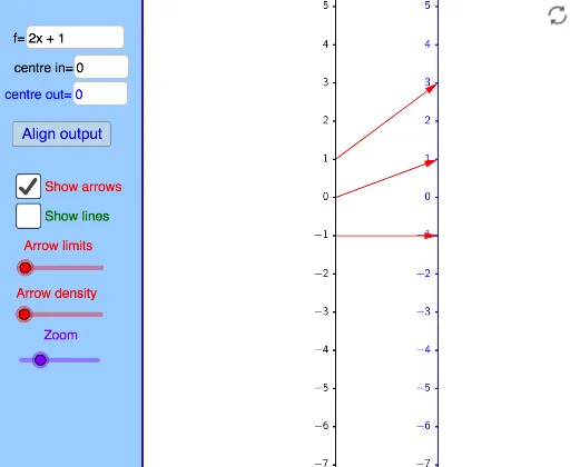
This example demonstrates how a function can be represented using a mapping diagram instead of a traditional graph, focusing on visualizing function mappings and relationships. It involves core mathematical concepts like function representation, mapping, and geometric intuition. The construction utilizes GeoGebra commands/objects such as TableText, Corner, Distance, Line, Text, panelleft1, Textfield, If, Sequence, Vector, Zip. It is suitable for high school mathematics education to understand different function representations and dynamic changes.
GeoGebra Commands & Parameters
TableText({{"0"}, {"\ \ \ \ \ \ \ \ \ \ \ \ \ \ \ \ "}}, "hc") → Xt0Corner(1) → corner1Corner(2) → corner2Corner(3) → corner3Corner(4) → corner4Corner(5) → screenDimDistance(corner1, corner2) → distXDistance(corner1, corner4) → distYLine(OY, yAxis) → YaxisLineText("(x,y) = (" + (x(A)) + "," + (y(A)) + ") in black coordinate system") → text2Text("(X,Y) = (" + (x(A) - x(OY)) + "," + (y(A) - y(OY)) + ") in blue coordinate system") → text1panelleft1(panelsize) → panelquad, panelseg1, panelseg2, panelseg3, panelseg4, panellineTextfield(f) → InputBox1Line(OX, yAxis) → XaxisLineTextfield(x0) → InputBox2If(minstepfrac > lg(5), 10^(minsteppower + 1), If[minstepfrac > lg(2), (5 * 10^(minsteppower)), If[minstepfrac > 0, (2 * 10^(minsteppower)), 10^(minsteppower)]]) → stepsizeSequence(Text[TableText[{{"\phantom{(}" + (x0 + (n * stepsize)) + ""}, {"\phantom{(} \ \ \ \ \ \ \ \ \ \ \ \ \ \ \ "}}, "hr"], (x(OX) - Distance[Corner[Xt0, 1], Corner[Xt0, 2]] + 7 / unitX, (n * steplength) + y(OX) + (Distance[Corner[Xt0, 1], Corner[Xt0, 4]] * 0.25) + 4 / unitY), true, true], n, ceil((y(Corner[1]) - y(OX)) / steplength), floor((y(Corner[4]) - y(OX)) / steplength)) → XaxisNumbersSequence(Segment[(x(OX), y(OX) + (n * steplength)), (x(OX) - 2 / unitX, y(OX) + (n * steplength))], n, ceil((y(Corner[1]) - y(OX)) / steplength), floor((y(Corner[4]) - y(OX)) / steplength)) → XaxisTicksSequence(Text[TableText[{{"\phantom{(}" + (y0 + (n * stepsize)) + ""}, {"\phantom{(} \ \ \ \ \ \ \ \ \ \ \ \ \ \ \ "}}, "hr"], (x(OY) - Distance[Corner[Xt0, 1], Corner[Xt0, 2]] + 7 / unitX, (n * steplength) + y(OY) + (Distance[Corner[Xt0, 1], Corner[Xt0, 4]] * 0.25) + 4 / unitY), true, true], n, ceil((y(Corner[1]) - y(OY)) / steplength), floor((y(Corner[4]) - y(OY)) / steplength)) → YaxisNumbersSequence(Segment[(x(OY), y(OY) + (n * steplength)), (x(OY) - 2 / unitX, y(OY) + (n * steplength))], n, ceil((y(Corner[1]) - y(OY)) / steplength), floor((y(Corner[4]) - y(OY)) / steplength)) → YaxisTicksVector((xpos, 0), (ypos, 0)) → uSequence(i / spacing, i, ((-numarrows) * spacing), (numarrows * spacing)) → arrowstartsZip(x0 + (as * numminstep), as, arrowstarts) → arrowxvalsZip(f(ax), ax, arrowxvals) → arrowyvalsZip((xpos, ((xv - x0) * steplength / stepsize)), xv, arrowxvals) → arrowxcoordsZip((ypos, ((yv - y0) * steplength / stepsize)), yv, arrowyvals) → arrowycoordsZip(Vector[ax, ay], ax, arrowxcoords, ay, arrowycoords) → arrowsZip(Line[ax, ay], ax, arrowxcoords, ay, arrowycoords) → linesTextfield(y0) → InputBox3Vector((xpos, 0), (ypos, ((f(x0) - y0) * steplength / stepsize))) → v
AI Drawing Prompt Reference
Create a visual mapping diagram for a function, showing two coordinate systems: a black one and a blue one. Display a point (x,y) in the black system and its corresponding (X,Y) in the blue system. Label the x and y axes with evenly spaced ticks. Use arrows to connect each x-value to its function output y-value, with the tail on the x-axis and head on the y-axis, in different colors for input and output. The diagram should clearly illustrate the function's mapping.
The prompt above was compiled from the original drawing commands and is for reference only.