
Mapping Diagrams - Composite Functions
Loading the math board and drawing, please wait…
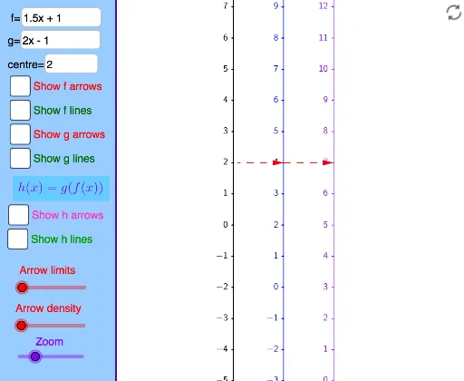
This example demonstrates how mapping diagrams represent the input-output relationships of composite functions. Core math concepts include function mapping, composite functions, and set correspondence. Construction highlights include commands like TableText, Line, Vector, and Sequence from GeoGebra to build dynamic diagrams. Ideal for high school students and teachers to visualize abstract function relationships and composite processes.
GeoGebra Commands & Parameters
TableText({{"0"}, {"\ \ \ \ \ \ \ \ \ \ \ \ \ \ \ \ "}}, "hc") → Xt0Corner(1) → corner1Corner(2) → corner2Corner(3) → corner3Corner(4) → corner4Corner(5) → screenDimDistance(corner1, corner2) → distXDistance(corner1, corner4) → distYLine(OY, yAxis) → YaxisLineText("(x,y) = (" + (x(A)) + "," + (y(A)) + ") in black coordinate system") → text2Text("(X,Y) = (" + (x(A) - x(OY)) + "," + (y(A) - y(OY)) + ") in blue coordinate system") → text1panelleft1(panelsize) → panelquad, panelseg1, panelseg2, panelseg3, panelseg4, panellineTextfield(f) → InputBox1Line(OX, yAxis) → XaxisLineTextfield(x0) → InputBox3If(minstepfrac > lg(5), 10^(minsteppower + 1), If[minstepfrac > lg(2), (5 * 10^(minsteppower)), If[minstepfrac > 0, (2 * 10^(minsteppower)), 10^(minsteppower)]]) → stepsizeSequence(Text[TableText[{{"\phantom{(}" + (x0 + (n * stepsize)) + ""}, {"\phantom{(} \ \ \ \ \ \ \ \ \ \ \ \ \ \ \ "}}, "hr"], (x(OX) - Distance[Corner[Xt0, 1], Corner[Xt0, 2]] + 7 / unitX, (n * steplength) + y(OX) + (Distance[Corner[Xt0, 1], Corner[Xt0, 4]] * 0.25) + 4 / unitY), true, true], n, ceil((y(Corner[1]) - y(OX)) / steplength), floor((y(Corner[4]) - y(OX)) / steplength)) → XaxisNumbersSequence(Segment[(x(OX), y(OX) + (n * steplength)), (x(OX) - 2 / unitX, y(OX) + (n * steplength))], n, ceil((y(Corner[1]) - y(OX)) / steplength), floor((y(Corner[4]) - y(OX)) / steplength)) → XaxisTicksSequence(Text[TableText[{{"\phantom{(}" + (y0 + (n * stepsize)) + ""}, {"\phantom{(} \ \ \ \ \ \ \ \ \ \ \ \ \ \ \ "}}, "hr"], (x(OY) - Distance[Corner[Xt0, 1], Corner[Xt0, 2]] + 7 / unitX, (n * steplength) + y(OY) + (Distance[Corner[Xt0, 1], Corner[Xt0, 4]] * 0.25) + 4 / unitY), true, true], n, ceil((y(Corner[1]) - y(OY)) / steplength), floor((y(Corner[4]) - y(OY)) / steplength)) → YaxisNumbersSequence(Segment[(x(OY), y(OY) + (n * steplength)), (x(OY) - 2 / unitX, y(OY) + (n * steplength))], n, ceil((y(Corner[1]) - y(OY)) / steplength), floor((y(Corner[4]) - y(OY)) / steplength)) → YaxisTicksVector((xpos, 0), (ypos, 0)) → uSequence(i / spacing, i, ((-numarrows) * spacing), (numarrows * spacing)) → arrowstartsZip(x0 + (as * numminstep), as, arrowstarts) → arrowxvalsZip(f(ax), ax, arrowxvals) → arrowyvalsZip((xpos, ((xv - x0) * steplength / stepsize)), xv, arrowxvals) → arrowxcoordsZip((ypos, ((yv - y0) * steplength / stepsize)), yv, arrowyvals) → arrowycoordsZip(Vector[ax, ay], ax, arrowxcoords, ay, arrowycoords) → farrowsZip(Line[ax, ay], ax, arrowxcoords, ay, arrowycoords) → flinesTextfield(g) → InputBox2Line(OZ, yAxis) → ZaxisLineSequence(Text[TableText[{{"\phantom{(}" + (z0 + (n * stepsize)) + ""}, {"\phantom{(} \ \ \ \ \ \ \ \ \ \ \ \ \ \ \ "}}, "hr"], (x(OZ) - Distance[Corner[Xt0, 1], Corner[Xt0, 2]] + 7 / unitX, (n * steplength) + y(OZ) + (Distance[Corner[Xt0, 1], Corner[Xt0, 4]] * 0.25) + 4 / unitY), true, true], n, ceil((y(Corner[1]) - y(OZ)) / steplength), floor((y(Corner[4]) - y(OZ)) / steplength)) → ZaxisNumbersSequence(Segment[(x(OZ), y(OZ) + (n * steplength)), (x(OZ) - 2 / unitX, y(OZ) + (n * steplength))], n, ceil((y(Corner[1]) - y(OZ)) / steplength), floor((y(Corner[4]) - y(OZ)) / steplength)) → ZaxisTicksZip(g(f(ax)), ax, arrowxvals) → arrowzvalsZip((zpos, ((zv - z0) * steplength / stepsize)), zv, arrowzvals) → arrowzcoordsZip(Vector[ay, az], ay, arrowycoords, az, arrowzcoords) → garrowsZip(Vector[ax, az], ax, arrowxcoords, az, arrowzcoords) → harrowsVector((ypos, 0), (zpos, 0)) → vZip(Line[ay, az], ay, arrowycoords, az, arrowzcoords) → glinesZip(Line[ax, az], ax, arrowxcoords, az, arrowzcoords) → hlines
AI Drawing Prompt Reference
Create a mapping diagram for composite functions, including two coordinate systems: one for function f and another for function g. Draw the graph of function f in the input coordinate system and the graph of function g in the output coordinate system. Use arrows to show the mapping relationship between input and output, with arrows pointing from the input coordinate system to the output coordinate system, illustrating the process of composite functions.
The prompt above was compiled from the original drawing commands and is for reference only.