
Equivalent Linear Equations Self-Practice
Loading the math board and drawing, please wait…
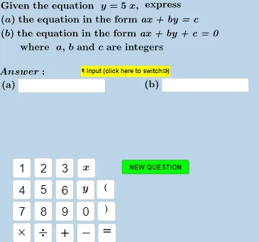
① This example is a self-practice activity designed to help students master the concept of equivalent linear equations, generating random problems and providing instant feedback. ② The core mathematical concept is equivalent linear equations, meaning equations that share the same solution set, typically obtained through algebraic manipulations such as adding, subtracting, multiplying, dividing, or rearranging terms. ③ Construction highlights: The GeoGebra construction uses random generation (Random, RandomElement), text processing (TextToUnicode, Join, Expand), conditional logic (If, CountIf), and interactive components (Textfield, Button) to dynamically create questions and check answers; objects include counters, variables a, b, c, and multiple text display areas. ④ Suitable for middle school to high school students, this can be used for classroom practice, self-study, or as a teacher's demonstration tool for illustrating equivalent equation transformations.
GeoGebra Commands & Parameters
If(counter < 2, RandomElement[{-5, -4, -3, -2, -1, 1, 2, 3, 4, 5}], If[counter < 3, RandomElement[{-6, -4, -2, 2, 4, 6}], If[counter < 4, RandomElement[{-9, -6, -3, 3, 6, 9}], RandomElement[{-6, -5, -4, -3, -2, -1, 1, 2, 3, 4, 5, 6, 7}]]]) → aIf(counter < 2, 1, If[counter < 3, 2, If[counter < 4, 3, RandomElement[{1, 2, 3, 4, 5, 6}]]]) → bIf(counter < 2, Random[-7, 9], If[counter < 3, RandomElement[{-10 - 8, -6, -4, -2, 2, 4, 6, 8, 10}], If[counter < 4, RandomElement[{-15, -12, -9, -6, -3, 3, 6, 9, 12, 15}], Random[-7, 9]]]) → c_1GCD({a, b, c_1}) → c_hTextToUnicode(Text[h]) → l3Sequence(32, k, 1, CountIf[x ≟ 32, TextToUnicode[Text[h_1]]]) → l3_sRemove(l3, l3_s) → l3_cTextToUnicode(textl32) → l32Sequence(32, k, 1, CountIf[x ≟ 32, l32]) → l32_sRemove(l32, l32_s) → l32_cTextToUnicode(textl22) → l22Sequence(32, k, 1, CountIf[x ≟ 32, l22]) → l22_sRemove(l22, l22_s) → l22_cExpand(Simplify[((-(x(g) / y(g))) * x) - z(g) / y(g)]) → f_1TextToUnicode(Text[f_1]) → l1Sequence(32, k, 1, CountIf[x ≟ 32, TextToUnicode[Text[f_1]]]) → l1_sJoin({TextToUnicode["y="], Remove[l1, l1_s]}) → l1_cTextToUnicode(Text[g]) → l2If(counter < 5, 1, If[counter < 8, 2, 3]) → typeRandom(-6, 7) → cGCD({a, b, c}) → c_gSequence(32, k, 1, CountIf[x ≟ 32, TextToUnicode[Text[g_1]]]) → l2_sRemove(l2, l2_s) → l2_cTextToUnicode(Text[textanswera]) → laSequence(32, k, 1, CountIf[x ≟ 32, la]) → la_sRemove(la, la_s) → la_cTextToUnicode(Text[eqb]) → lbbSequence(32, k, 1, CountIf[x ≟ 32, lbb]) → lbb_sRemove(lbb, lbb_s) → lbb_cTextToUnicode(Text[eqa]) → laaSequence(32, k, 1, CountIf[x ≟ 32, laa]) → laa_sRemove(laa, laa_s) → laa_cTextToUnicode(Text[textanswerb]) → lbSequence(32, k, 1, CountIf[x ≟ 32, lb]) → lb_sRemove(lb, lb_s) → lb_cRandomElement({-5, -4, -3, -2, 1, 0, 1, 2, 3, 4, 5, 1 / 2, 1 / 3, 1 / 4, 3 / 4, 1 / 5, 2 / 3, 1 / 5, 2 / 5, 3 / 5, 4 / 5, -1 / 2, -1 / 3, -1 / 4, -3 / 4, -1 / 5, -2 / 3, -1 / 5, -2 / 5, -3 / 5, -4 / 5}) → mExpand(Simplify[(m * x) + c]) → fIf(type < 2, la_c ≟ l2_c ∨ la_c ≟ l22_c, If[type ≟ 2, la_c ≟ l3_c ∨ la_c ≟ l32_c, la_c ≟ l1_c]) → answeracorrectIf(type ≟ 1, m, If[type ≟ 2, m_d, m_d]) → m_sIf(type ≟ 1, c, c_d) → c_sIf(type < 2, lb_c ≟ l3_c ∨ lb_c ≟ l32_c, If[type ≟ 2, lb_c ≟ l1_c ∨ lb_c ≟ l1_c, lb_c ≟ l2_c ∨ lb_c ≟ l22_c]) → answerbcorrectTextfield(textanswera) → InputBox1Textfield(textanswerb) → InputBox2Expand(Simplify[(m_s * x) + c_s]) → f_sCountIf(x ≟ 32, {32, 32, 35, 34, 56}) → dPoint(g, 0.3) → BPoint(g, 0.7) → A
AI Drawing Prompt Reference
Create an interactive graphic showing the equivalence of randomly generated linear equations. Include sliders to control parameters, dynamically generating and displaying the equations. Key elements: graphs of two linear equations, parameter sliders, text areas for equations, input boxes for answers, and a button to check answers. First, plot the graphs of the two linear equations, then use sliders to adjust parameters and observe changes in the graphs, finally displaying the equations and answers in text areas.
The prompt above was compiled from the original drawing commands and is for reference only.