
Equation Balance Model
Loading the math board and drawing, please wait…
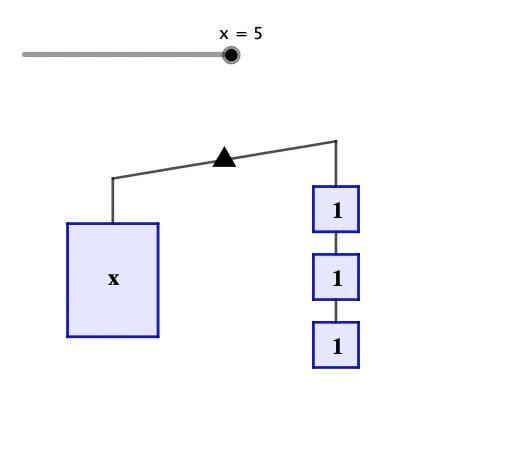
This example demonstrates a dynamic model where students modify variable values to observe changes in equation balance. Core math concepts include equation equilibrium, variable impact, and analytical geometry. Constructed using commands like Segment, Circle, Intersect, Line, OrthogonalLine, Polygon, Point in GeoGebra, suitable for high school mathematics teaching to understand the geometric meaning of equation solutions and the effects of parameter changes.
GeoGebra Commands & Parameters
Segment(C, B) → fCircle(A, 2.5) → cIntersect(c, f, 1) → DIntersect(c, f, 2) → ESegment(D, E) → gLine(E, eq1) → hLine(D, eq1) → iCircle(E, 1) → dCircle(D, 1) → eIntersect(e, i, 2) → FIntersect(d, h, 2) → GCircle(G, 1.5) → kIntersect(k, h, 2) → HCircle(H, 1.5) → pIntersect(p, h, 2) → IOrthogonalLine(F, i) → jOrthogonalLine(G, h) → lOrthogonalLine(H, h) → mOrthogonalLine(I, h) → nCircle(G, 0.5) → qCircle(H, 0.5) → rCircle(I, 0.5) → sIntersect(q, l, 1) → JIntersect(q, l, 2) → KIntersect(r, m, 1) → LIntersect(r, m, 2) → MIntersect(s, n, 1) → NIntersect(s, n, 2) → OOrthogonalLine(K, l) → tOrthogonalLine(J, l) → bCircle(J, 1) → c_1Circle(K, 1) → d_1Circle(L, 1) → e_1Circle(M, 1) → f_1Circle(N, 1) → g_1Circle(O, 1) → h_1Intersect(c_1, b, 1) → PIntersect(d_1, t, 1) → QIntersect(e_1, b, 1) → RIntersect(f_1, t, 1) → SIntersect(g_1, b, 1) → TIntersect(h_1, t, 1) → USegment(E, G) → i_1Segment(J, K) → j_1Segment(K, Q) → k_1Segment(Q, P) → l_1Segment(P, J) → m_1Segment(L, M) → n_1Segment(R, S) → p_1Segment(M, S) → q_1Segment(L, R) → r_1Segment(N, T) → s_1Segment(N, O) → t_1Segment(O, U) → a_1Segment(U, T) → b_1Intersect(h, l_1) → VIntersect(h, p_1) → WSegment(V, H) → f_2Segment(W, I) → g_2Circle(F, a / 5) → c_2Intersect(c_2, j, 1) → ZIntersect(c_2, j, 2) → A_1OrthogonalLine(A_1, j) → h_2OrthogonalLine(Z, j) → i_2Circle(A_1, 2.5) → d_2Circle(Z, 2.5) → e_2Intersect(e_2, i_2, 1) → B_1Intersect(d_2, h_2, 1) → C_1Segment(D, F) → j_2Segment(Z, A_1) → k_2Segment(A_1, C_1) → l_2Segment(C_1, B_1) → m_2Segment(B_1, Z) → n_2Polygon(Z, A_1, C_1, B_1) → q1, z_1, p_2, q_2, r_2Polygon(P, J, K, Q) → q2, p_3, j_3, k_3, q_3Polygon(L, M, S, R) → q3, l_3, m_3, s_2, r_3Polygon(N, O, U, T) → q4, n_3, o, u, t_2Circle(P, 0.3) → c_3Intersect(c_3, m_1, 1) → D_1Line(D_1, l_1) → a_2Circle(D_1, 0.4) → d_3Intersect(d_3, a_2, 1) → E_1Circle(R, 0.3) → e_3Intersect(e_3, r_1, 1) → F_1Circle(F_1, 0.4) → f_3Line(F_1, p_1) → b_2Intersect(f_3, b_2, 2) → G_1Circle(T, 0.3) → g_3Intersect(g_3, s_1, 1) → H_1Circle(H_1, 0.4) → h_3Line(H_1, b_1) → i_3Intersect(h_3, i_3, 1) → I_1Point(n_2) → J_1Circle(B_1, J_1) → s_3Line(J_1, m_2) → t_3Intersect(i, t_3) → K_1Circle(K_1, 0.1) → c_4Intersect(c_4, t_3, 2) → L_1