Electric Field Vectors: Superposition and Geometric Construction

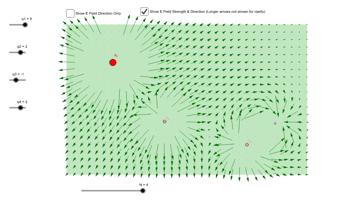
This GeoGebra example visualizes the electric field vector distribution generated by multiple point charges, demonstrating how field strength and direction vary across space. The core mathematical concepts include vector superposition, Coulomb's law in vector form, similar triangles used for vector decomposition, and sequence-based generation of a vector field. Construction highlights: commands such as Intersect, Point, Polygon, PointIn, and Sequence are used to build the geometric framework and sample points; charge objects q1 to q4 are defined, with intermediate variables E1x, E2x, etc., computing individual field components, then combined into total field components Ex and Ey, and finally displayed as vector E with controls Efx, Egy, and a button1 for interactive toggling. Suitable for high school or introductory university physics courses on electric fields, as well as mathematics lessons on vector operations and geometric construction, offering a cross-disciplinary approach to understanding vector field visualization.