
Dynamic Visualization of Trigonometric Functions and the Unit Circle
Loading the math board and drawing, please wait…
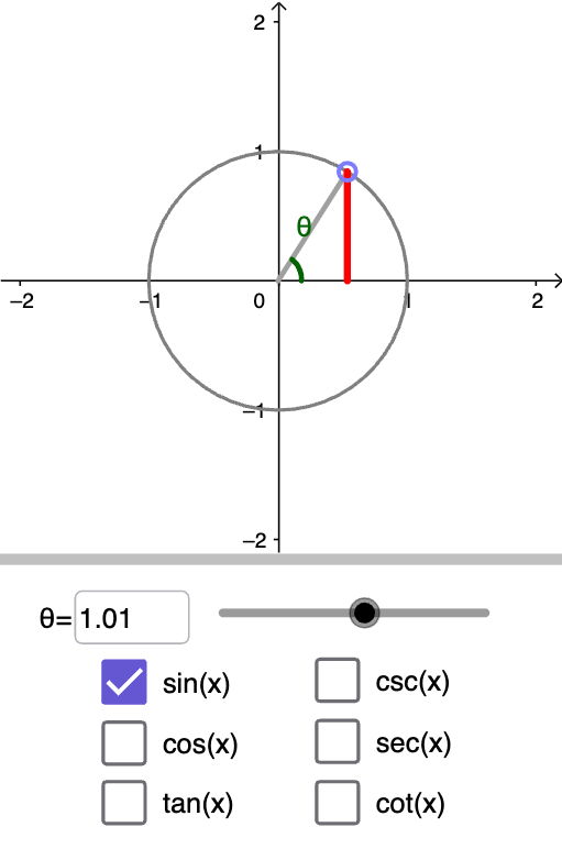
① This GeoGebra example presents an interactive unit circle that dynamically illustrates how sine, cosine, and other trigonometric values change with the angle, while simultaneously plotting the corresponding function curves. ② Core mathematical concepts include the definitions of trigonometric functions, the unit circle, angle and radian measures, transformations of function graphs, and trigonometric identities. ③ Construction highlights: using GeoGebra commands such as Circle to draw the unit circle, CurveCartesian for function curves, Slider to control the angle variable, Segment and Ray for radii and terminal sides, OrthogonalLine and Intersect to construct perpendiculars and intersections, Textfield and FractionText to display values and fractions, Element and If for dynamic lists, plus auxiliary objects like equilateral triangles, parabolas, and exponential functions for extended comparisons. ④ Suitable for high school and pre-university mathematics teaching, this resource helps students intuitively grasp periodicity, symmetry, and graph properties of trigonometric functions, and serves as an interactive tool for teacher demonstrations or student-led exploration.
GeoGebra Commands & Parameters
If(vals ≟ 8, "-", If[vals ≟ 24 ∨ vals ≟ 16, ""]) → textaux1'Element(functions, var) → FIf(val2 ≟ val2, Text[val2], "Undefined") → text6Element(values, vals) → EspvalFractionText(Espval) → textaux3If(vals ≟ 16, textaux1', textaux2) → text1If(vals ≟ 24 ∨ vals ≟ 8, textaux1', textaux3) → textaux4Circle((0, 0), 1) → cIf(special ≟ true, Rotate[A, (Espval * pi), (0, 0)], Rotate[A, theta, (0, 0)]) → A'Segment((0, 0), A') → radiusIf(special ≟ true, ((Espval * pi), F((Espval * pi))), (theta, F(theta))) → BIf(special ≟ true, (Espval * pi), theta) → anglecurveCurveCartesian(((a * b^(i)) * cos(i)), ((a * b^(i)) * sin(i)), i, 0, anglecurve) → anglepositiveCurveCartesian(((a * b^(i)) * cos(i)), (((-a) * b^(i)) * sin(i)), i, 0, (-anglecurve)) → anglenegativeIf(special ≟ false, (4 * pi) + 0.5, (11 / 6 * pi) + 0.5) → xmaxIf(special ≟ true ∧ (a1 ≟ true ∨ a2 ≟ true ∨ a4 ≟ true ∨ a5 ≟ true), 3, If[special ≟ false ∧ (a3 ≟ true ∨ a6 ≟ true), 8.5, 4.5]) → ymaxIf(special ≟ true ∧ (a1 ≟ true ∨ a2 ≟ true), 4, 6) → dIf(special ≟ true ∧ (a1 ≟ true ∨ a2 ≟ true), 2, If[special ≟ false, 6, 16]) → auxIf(val1 ≟ val1, SurdText[val1], "Undefined") → surd1If(special ≟ true, Segment[((Espval * pi), 0), B], Segment[(theta, 0), B]) → fIf(val1 ≟ val1, SurdText[val1], "Undefined") → text4Segment((x(A'), 0), A') → seg1Segment((0, y(A')), A') → seg2Line((0, 0), A') → gOrthogonalLine((1, 0), xAxis) → hOrthogonalLine((-1, 0), xAxis) → iIntersect(g, h) → COrthogonalLine((0, 1), yAxis) → jOrthogonalLine((0, -1), yAxis) → kIntersect(g, j) → DSegment((1, 0), C) → seg3Segment((0, 1), D) → seg6Segment((0, 0), D) → seg4Segment((0, 0), C) → seg5Tangent(A', c) → l,Intersect(xAxis, l) → EIntersect(yAxis, l) → GSegment(A', E) → seg3'Segment((0, 0), G) → seg4'Segment((0, 0), E) → seg5'Segment(G, A') → seg6'Ray((0, 0), A') → mSegment(G, E) → nTextfield(theta) → InputBox1If(special ≟ true, (180 * ° / 3), 180°) → divgradIf(special ≟ true, pi / 2, pi) → divPoint(yAxis) → HOrthogonalLine(H, yAxis) → pElement(thetaRadians, vals) → NewIf(a1 ≟ true, text2, If[a2 ≟ true, text7, If[a3 ≟ true, text14, If[a4 ≟ true, text17, If[a5 ≟ true, text16, If[a6 ≟ true, text15]]]]]) → func
AI Drawing Prompt Reference
Draw a unit circle and dynamically show the angle θ and its corresponding sine and cosine values. First, draw a circle with radius 1, then add a slider to control the angle, find the corresponding point A on the circle, draw a line segment from the origin to point A to represent the radius, and draw vertical and horizontal lines to show the sine and cosine values, and use curves to represent the sine and cosine functions.
The prompt above was compiled from the original drawing commands and is for reference only.