
Distribution Comparison
Loading the math board and drawing, please wait…
In collections
Statistical Intuition Builders
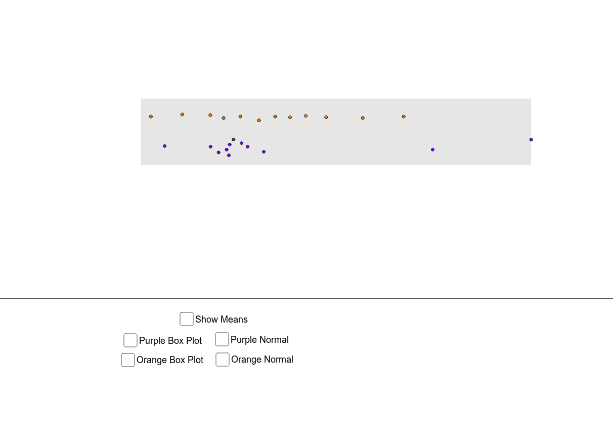
This example demonstrates how to compare and contrast statistical measures of center (like mean, median) and data displays (like box plots, scatter plots) across different datasets. It visually illustrates concepts such as normal distribution and standard deviation through dynamic manipulation. Key construction elements include commands like Polygon, PointIn, BoxPlot, MeanX, SDX, Normal, Intersect, Circle, OrthogonalLine, Segment, Mirror, and objects like poly1, a, top, c, mid, etc. Suitable for high school and above mathematics education, particularly in probability & statistics and data analysis courses.
GeoGebra Commands & Parameters
Polygon(A, B, C, D) → poly1, a, top, c, midPolygon(E, F, G, H) → poly2, e, bottom, g, hPointIn(poly1) → PPointIn(poly1) → QPointIn(poly1) → RPointIn(poly1) → OPointIn(poly1) → A_1PointIn(poly1) → B_1PointIn(poly1) → IPointIn(poly1) → JPointIn(poly1) → KPointIn(poly1) → LPointIn(poly1) → MPointIn(poly1) → NPointIn(poly2) → SPointIn(poly2) → TPointIn(poly2) → UPointIn(poly2) → VPointIn(poly2) → WPointIn(poly2) → ZPointIn(poly2) → C_1PointIn(poly2) → D_1PointIn(poly2) → E_1PointIn(poly2) → F_1PointIn(poly2) → G_1PointIn(poly2) → H_1BoxPlot(7.5, 0.3, x(list_o), true) → boxorangeBoxPlot(6.5, 0.3, x(list_p), true) → boxpurpleMeanX(list_o) → mean_oMeanX(list_p) → mean_pSDX(list_o) → sd_oSDX(list_p) → sd_pNormal(mean_o, sd_o, x) → fNormal(mean_p, sd_p, x) → pIntersect(d, xAxis) → I_1Intersect(b, xAxis) → J_1Circle(I_1, sd_p) → kCircle(I_1, (2 * sd_p)) → sCircle(I_1, (3 * sd_p)) → tCircle(J_1, sd_o) → c_1Circle(J_1, (2 * sd_o)) → d_1Circle(J_1, (3 * sd_o)) → e_1Intersect(k, xAxis) → K_1, L_1Intersect(s, xAxis) → M_1, N_1Intersect(t, xAxis) → O_1, P_1OrthogonalLine(K_1, xAxis) → iOrthogonalLine(M_1, xAxis) → jOrthogonalLine(O_1, xAxis) → lOrthogonalLine(L_1, xAxis) → mOrthogonalLine(N_1, xAxis) → nOrthogonalLine(P_1, xAxis) → a_1Circle(I_1, 6.5) → f_1Intersect(f_1, d) → Q_1, R_1Intersect(r, d, (-3.774228689632889, 2.1243967656986413)) → S_1Intersect(r, i, (-9.407954274837792, 1.2885117717905816)) → T_1Intersect(r, j, (-15.041679860042695, 0.2875058379927696)) → U_1Intersect(r, l, (-20.6754054452476, 0.023599916315999357)) → V_1Intersect(r, m, (1.8594968955720141, 1.2885117717905816)) → W_1Intersect(r, n, (7.493222480776917, 0.2875058379927696)) → Z_1Intersect(r, a_1, (13.126948065981821, 0.023599916315999357)) → A_2Segment(M_1, U_1) → b_1Segment(N_1, Z_1) → j_1Segment(P_1, A_2) → k_1Segment(I_1, Q_1) → h_1Segment(O_1, V_1) → l_1Circle(J_1, 7.5) → p_1Intersect(p_1, b) → B_2, C_2Segment(J_1, B_2) → m_1OrthogonalLine(D_2, xAxis) → n_1OrthogonalLine(E_2, xAxis) → q_1OrthogonalLine(F_2, xAxis) → r_1Mirror(n_1, m_1) → s_1Mirror(q_1, m_1) → t_1Mirror(r_1, m_1) → a_2Intersect(q, s_1, (-7.75562250181825, 1.8221829408666963)) → G_2Intersect(s_1, xAxis) → H_2Intersect(t_1, xAxis) → I_2Intersect(q, t_1, (-11.739372745974084, 0.4065839714153232)) → J_2Intersect(a_2, xAxis) → K_2Intersect(q, a_2, (-15.72312299012992, 0.03337444473412614)) → L_2Intersect(q, n_1, (0.21187798649342193, 1.8221829408666963)) → M_2Intersect(q, q_1, (4.195628230649257, 0.4065839714153229)) → N_2Intersect(q, r_1, (8.179378474805093, 0.03337444473412608)) → O_2Segment(K_2, L_2) → b_2Segment(I_2, J_2) → c_2Segment(N_2, E_2) → d_2Segment(O_2, F_2) → e_2OrthogonalLine(L_1, top) → i_2Intersect(i_2, top) → P_2OrthogonalLine(K_1, top) → j_2Intersect(top, j_2) → Q_2Segment(K_1, Q_2) → g_1Segment(L_1, P_2) → i_1OrthogonalLine(H_2, top) → k_2OrthogonalLine(D_2, top) → l_2Intersect(k_2, top) → R_2Intersect(l_2, top) → S_2Segment(H_2, R_2) → f_2Segment(D_2, S_2) → g_2