
Disc Method Calculus Demo
Loading the math board and drawing, please wait…
In collections
GeoGebra 3D & AR: PreCalc & Calculus Resources
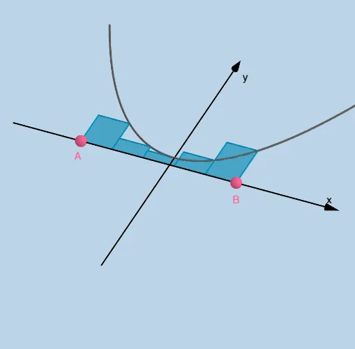
This example demonstrates the geometric process of calculating the volume of a solid of revolution using the disc method. It involves core calculus concepts like integration, volume calculation, and geometric transformations. Key GeoGebra commands and objects used include Polygon, Surface, RectangleSum, Sequence, Rotate, and Textfield for dynamic visualization and volume computation, suitable for high school students and calculus beginners.
GeoGebra Commands & Parameters
Polygon(A, B, D, C) → q1, a_1, b_1, d, cSurface(1 + u, (y(C) * cos(v)), (y(C) * sin(v)), u, 0, 1, v, 0, α) → eSurface(x(B), ((u * y(D)) * cos(v)), ((u * y(D)) * sin(v)), u, 0, 1, v, 0, α) → fSurface(x(A), ((u * y(D)) * cos(v)), ((u * y(D)) * sin(v)), u, 0, 1, v, 0, α) → gRectangleSum(h, a, b, n, q) → iSequence(Polygon[(a + (i * deltax), 0), (a + ((i + 1) * deltax), 0), (a + ((i + 1) * deltax), h(a + ((i + 1) * deltax))), (a + (i * deltax), h(a + ((i + 1) * deltax)))], i, 0, n - 1) → L_1Sequence(Surface[a + (i * deltax) + (deltax * u), (h(a + ((i + 1) * deltax)) * cos(v)), (h(a + ((i + 1) * deltax)) * sin(v)), u, 0, 1, v, 0, α], i, 0, n - 1, 1) → L_4Sequence(Surface[a + (i * deltax), ((h(a + ((i + 1) * deltax)) * cos(v)) * u), ((h(a + ((i + 1) * deltax)) * sin(v)) * u), u, 0, 1, v, 0, α], i, 0, n - 1, 1) → L_2Sequence(Surface[a + ((i + 1) * deltax), ((h(a + ((i + 1) * deltax)) * cos(v)) * u), ((h(a + ((i + 1) * deltax)) * sin(v)) * u), u, 0, 1, v, 0, α], i, 0, n - 1, 1) → L_3Rotate(L_1, α, xAxis) → L_5Textfield(a) → InputBox1Textfield(b) → InputBox2Textfield(n) → InputBox3Textfield(h) → InputBox4
AI Drawing Prompt Reference
Draw a solid of revolution formed by rotating a given function around the x-axis and calculate its volume using the rectangular approximation method. First, draw a quadrilateral, then rotate it around the x-axis to generate the surface of the solid. Next, use the rectangular approximation method by rotating a series of rectangles to approximate the volume of the solid. Finally, input the function expression, interval, and number of divisions through input boxes to dynamically adjust the shape and volume approximation of the solid.
The prompt above was compiled from the original drawing commands and is for reference only.