
Direction Fields and Solution Curves
Loading the math board and drawing, please wait…
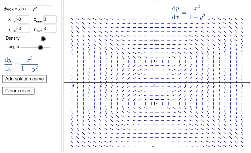
This example illustrates direction fields and solution curves for a first-order differential equation. It involves concepts like differential equations, direction fields, and loci. Construction uses GeoGebra commands such as SlopeField, Locus, and If. Suitable for high school students or college undergraduates learning calculus and coordinate geometry.
GeoGebra Commands & Parameters
Textfield(f) → inputBox1Textfield(x_{min}) → inputBox2Textfield(x_{max}) → inputBox3Textfield(y_{min}) → inputBox4Textfield(y_{max}) → inputBox5SlopeField(f, n, L, x_{min}, y_{min}, x_{max}, y_{max}) → slopefield1Locus(f(x, y), A) → numericalIntegral1Locus(f(x, y), B) → bcLocus(f(x, y), C) → ccLocus(f(x, y), D) → dcLocus(f(x, y), E) → ecLocus(f(x, y), F) → fcLocus(f(x, y), G) → gcLocus(f(x, y), H) → hcLocus(f(x, y), I) → icLocus(f(x, y), J) → jcIf(x_{min} < 0, 0, x_{min}) → x0If(x_{min} > 0, x_{min}, 0) → xm