
Direction Fields and Solution Curves by Dr. Doug Davis, 3D
Loading the math board and drawing, please wait…
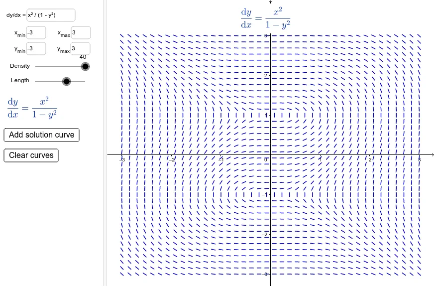
This example demonstrates the slope field and solution curves of a first-order differential equation. Key mathematical concepts include differential equations and curve sketching. Commands used include text field, slope field, locus, and more. Suitable for calculus and ordinary differential equations courses.
GeoGebra Commands & Parameters
Textfield(f) → inputBox1Textfield(x_{min}) → inputBox2Textfield(x_{max}) → inputBox3Textfield(y_{min}) → inputBox4Textfield(y_{max}) → inputBox5SlopeField(f, n, L, x_{min}, y_{min}, x_{max}, y_{max}) → slopefield1Locus(f(x, y), A) → numericalIntegral1Locus(f(x, y), B) → bcLocus(f(x, y), C) → ccLocus(f(x, y), D) → dcLocus(f(x, y), E) → ecLocus(f(x, y), F) → fcLocus(f(x, y), G) → gcLocus(f(x, y), H) → hcLocus(f(x, y), I) → icLocus(f(x, y), J) → jcIf(x_{min} > 0, x_{min}, 0) → xmTextfield(f_1) → inputBox1_1Textfield(f_2) → inputBox1_2
AI Drawing Prompt Reference
Create a slope field and several solution curves for a first-order differential equation. Begin by displaying the slope field across the coordinate plane, using short line segments to indicate tangent directions at each point. Then, from multiple distinct starting points, draw solution curves that smoothly follow the field, each taking a different path based on its initial condition. Additionally, include adjustable input boxes around the plot for modifying the equation and the x- and y-axis ranges, allowing dynamic exploration of how the field and curves change. The overall layout should be clear for analyzing the geometric behavior of the differential equation.
The prompt above was compiled from the original drawing commands and is for reference only.