
Demonstration of a Set of Two Linear First Order Differential Equations
Loading the math board and drawing, please wait…
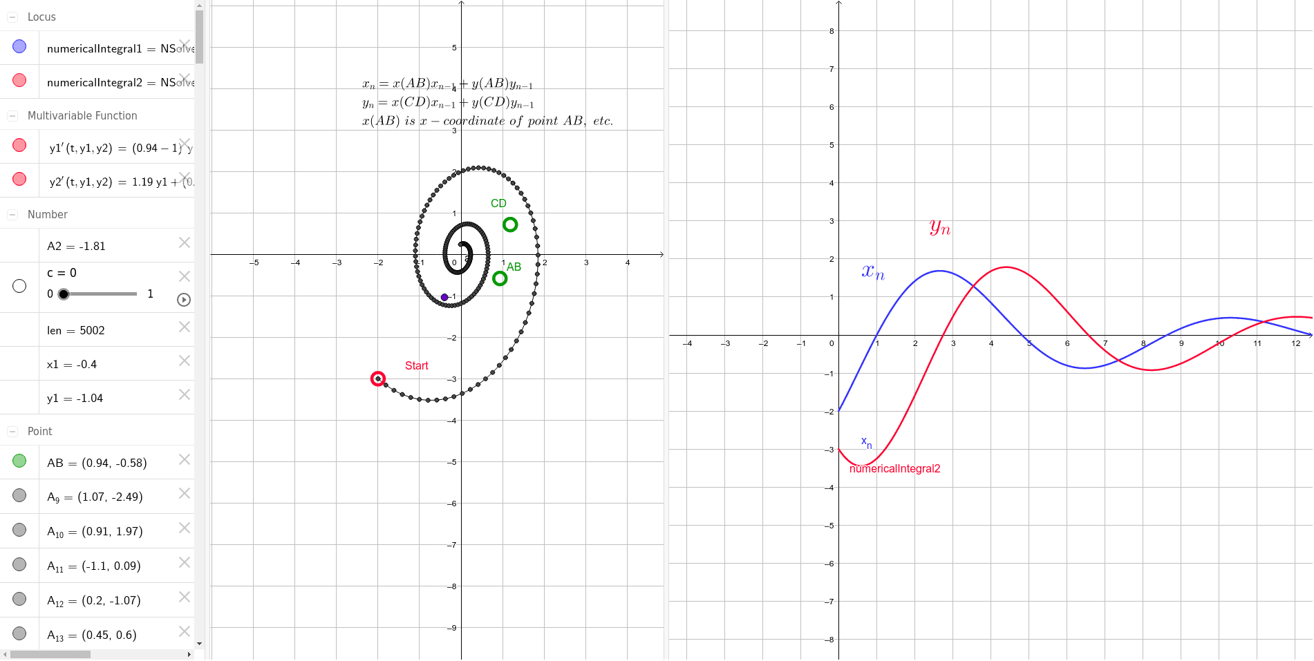
This example demonstrates the numerical solutions and integral curves of a set of two linear first-order differential equations. It involves core mathematical concepts such as differential equations, numerical solution methods (NSolveODE), integral curves, and analytical geometry. The construction utilizes GeoGebra commands like NSolveODE for solving differential equations, Length for calculating lengths, and PolyLine for drawing curves, along with objects like Start, AB, CD, y1', y2', numericalIntegral1, numericalIntegral2, c, y1, x1, A1-B15 for parameter settings and graphical representation. It is suitable for high school and above students to learn and understand the numerical solution methods and graphical representation of differential equations, and can be used for teaching demonstrations and exploratory learning.
GeoGebra Commands & Parameters
NSolveODE({y1', y2'}, 0, {x(Start), y(Start)}, 50) → numericalIntegral1, numericalIntegral2Length(numericalIntegral1) → lenPolyLine({I_8, J_8, K_8, L_8, M_8, N_8, O_8, P_8, Q_8, R_8, S_8, T_8, U_8, V_8, W_8, Z_8, A_9, B_9, C_9, D_9, E_9, F_9, G_9, H_9, I_9, J_9, K_9, L_9, M_9, N_9, O_9, P_9, Q_9, R_9, S_9, T_9, U_9, V_9, W_9, Z_9, A_{10}, B_{10}, C_{10}, D_{10}, E_{10}, F_{10}, G_{10}, H_{10}, I_{10}, J_{10}, K_{10}, L_{10}, M_{10}, N_{10}, O_{10}, P_{10}, Q_{10}, R_{10}, S_{10}, T_{10}, U_{10}, V_{10}, W_{10}, Z_{10}, A_{11}, B_{11}, C_{11}, D_{11}, E_{11}, F_{11}, G_{11}, H_{11}, I_{11}, J_{11}, K_{11}, L_{11}, M_{11}, N_{11}, O_{11}, P_{11}, Q_{11}, R_{11}, S_{11}, T_{11}, U_{11}, V_{11}, W_{11}, Z_{11}, A_{12}, B_{12}, C_{12}, D_{12}, E_{12}, F_{12}, G_{12}, H_{12}, I_{12}, J_{12}, K_{12}, L_{12}, M_{12}, N_{12}, O_{12}, P_{12}, Q_{12}, R_{12}, S_{12}, T_{12}, U_{12}, V_{12}, W_{12}, Z_{12}, A_{13}, B_{13}, C_{13}, D_{13}, E_{13}, F_{13}, G_{13}, H_{13}, I_{13}, J_{13}, K_{13}, L_{13}, M_{13}, N_{13}, O_{13}, P_{13}, Q_{13}, R_{13}, S_{13}, T_{13}, U_{13}, V_{13}, W_{13}, Z_{13}, A_{14}, B_{14}, C_{14}, D_{14}, E_{14}, F_{14}, G_{14}, H_{14}, I_{14}, J_{14}, K_{14}, L_{14}, M_{14}, N_{14}, O_{14}, P_{14}, Q_{14}, R_{14}, S_{14}, T_{14}, U_{14}, V_{14}, W_{14}, Z_{14}, A_{15}, B_{15}, C_{15}, D_{15}, E_{15}, F_{15}, G_{15}, H_{15}, I_{15}, J_{15}, K_{15}, L_{15}, M_{15}, N_{15}, O_{15}, P_{15}, Q_{15}, R_{15}, S_{15}, T_{15}, U_{15}, V_{15}, W_{15}, Z_{15}, A_{16}, B_{16}, C_{16}, D_{16}, E_{16}, F_{16}, G_{16}, H_{16}, I_{16}, J_{16}, K_{16}, L_{16}, M_{16}, N_{16}, O_{16}, P_{16}}) → a
AI Drawing Prompt Reference
Draw the numerical solutions and integral curves of a set of two linear first-order differential equations, showing the numerical solution methods, use different colored curves to represent at least two integral curves, starting from a point and passing through multiple points to the end point, the length of the curves can be distinguished by different colors or thicknesses, presenting a geometric representation effect in mathematical analysis.
The prompt above was compiled from the original drawing commands and is for reference only.