
Exploring a Set of Linear First Order Differential Equations
Loading the math board and drawing, please wait…
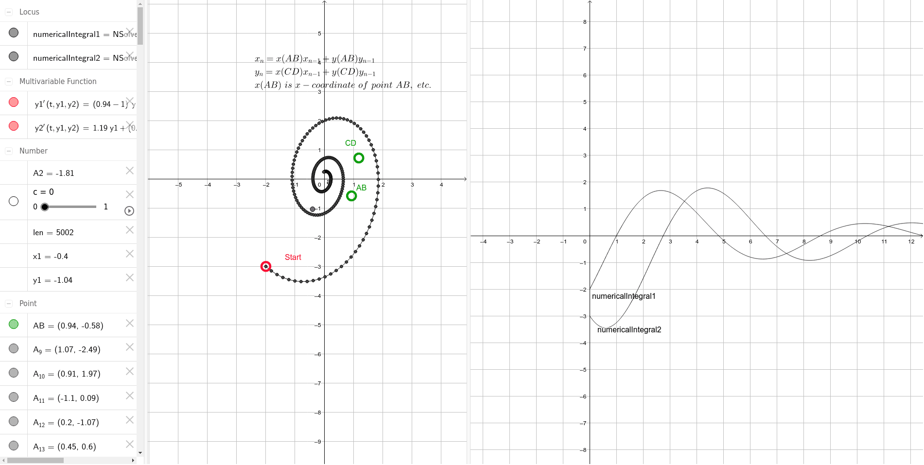
This example demonstrates how to use GeoGebra to explore a set of linear first order differential equations and the effects of their coefficients and initial positions. Key math concepts include differential equations, derivatives, and numerical integration. Construction highlights involve commands like NSolveODE for solving ODEs, Length for calculating lengths, and PolyLine for drawing lines, along with objects such as Start, AB, y1', CD, y2', numericalIntegral1, numericalIntegral2, c, y1, x1, A1, B1, A2, B2, A3, B3, A4, B4, A5, B5, A6, B6, A7, B7, A8, B8, A9, B9, A10, B10, A11, B11, A12, B12, A13, B13, A14, B14, A15, B15. Suitable for high school and above students to learn and understand the applications of differential equations.
GeoGebra Commands & Parameters
NSolveODE({y1', y2'}, 0, {x(Start), y(Start)}, 50) → numericalIntegral1, numericalIntegral2Length(numericalIntegral1) → lenPolyLine({I_8, J_8, K_8, L_8, M_8, N_8, O_8, P_8, Q_8, R_8, S_8, T_8, U_8, V_8, W_8, Z_8, A_9, B_9, C_9, D_9, E_9, F_9, G_9, H_9, I_9, J_9, K_9, L_9, M_9, N_9, O_9, P_9, Q_9, R_9, S_9, T_9, U_9, V_9, W_9, Z_9, A_{10}, B_{10}, C_{10}, D_{10}, E_{10}, F_{10}, G_{10}, H_{10}, I_{10}, J_{10}, K_{10}, L_{10}, M_{10}, N_{10}, O_{10}, P_{10}, Q_{10}, R_{10}, S_{10}, T_{10}, U_{10}, V_{10}, W_{10}, Z_{10}, A_{11}, B_{11}, C_{11}, D_{11}, E_{11}, F_{11}, G_{11}, H_{11}, I_{11}, J_{11}, K_{11}, L_{11}, M_{11}, N_{11}, O_{11}, P_{11}, Q_{11}, R_{11}, S_{11}, T_{11}, U_{11}, V_{11}, W_{11}, Z_{11}, A_{12}, B_{12}, C_{12}, D_{12}, E_{12}, F_{12}, G_{12}, H_{12}, I_{12}, J_{12}, K_{12}, L_{12}, M_{12}, N_{12}, O_{12}, P_{12}, Q_{12}, R_{12}, S_{12}, T_{12}, U_{12}, V_{12}, W_{12}, Z_{12}, A_{13}, B_{13}, C_{13}, D_{13}, E_{13}, F_{13}, G_{13}, H_{13}, I_{13}, J_{13}, K_{13}, L_{13}, M_{13}, N_{13}, O_{13}, P_{13}, Q_{13}, R_{13}, S_{13}, T_{13}, U_{13}, V_{13}, W_{13}, Z_{13}, A_{14}, B_{14}, C_{14}, D_{14}, E_{14}, F_{14}, G_{14}, H_{14}, I_{14}, J_{14}, K_{14}, L_{14}, M_{14}, N_{14}, O_{14}, P_{14}, Q_{14}, R_{14}, S_{14}, T_{14}, U_{14}, V_{14}, W_{14}, Z_{14}, A_{15}, B_{15}, C_{15}, D_{15}, E_{15}, F_{15}, G_{15}, H_{15}, I_{15}, J_{15}, K_{15}, L_{15}, M_{15}, N_{15}, O_{15}, P_{15}, Q_{15}, R_{15}, S_{15}, T_{15}, U_{15}, V_{15}, W_{15}, Z_{15}, A_{16}, B_{16}, C_{16}, D_{16}, E_{16}, F_{16}, G_{16}, H_{16}, I_{16}, J_{16}, K_{16}, L_{16}, M_{16}, N_{16}, O_{16}, P_{16}}) → a
AI Drawing Prompt Reference
Draw the solutions of a set of linear first-order differential equations, showing the effects of coefficients and initial positions. Use numerical integration to solve the differential equations, calculate the length of the integral paths, and connect the points on the integral paths with polylines to form continuous curves. Observe the changes in the solutions of the differential equations over time and the impact of coefficients on the solutions.
The prompt above was compiled from the original drawing commands and is for reference only.