
Definite Integral and Poisson Distribution
Loading the math board and drawing, please wait…
In collections
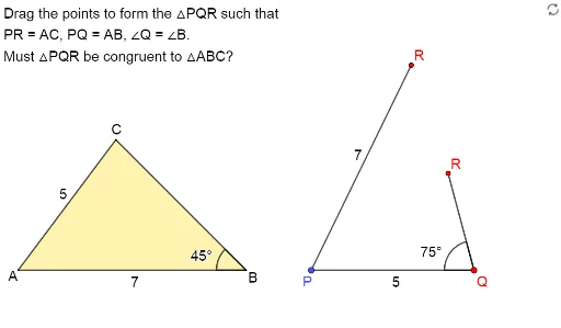
Exploring the Conditions for Congruence of 2 Triangles
Exploring Congruence of Triangles
This example illustrates the relationship between definite integrals and the Poisson distribution. It uses dynamic coordinates and vectors to demonstrate how to calculate the integral of a probability distribution function. Commands like Point, Vector, Sequence, and DynamicCoordinates are employed. Suitable for high school mathematics, particularly calculus and probability statistics courses.
GeoGebra Commands & Parameters
Point(Sequence[A + (i, 0), i, 1, 20, 1]) → BVector(A, C1) → uSequence(A + (i * UnitVector[Segment[A, C1]]), i, 1, 20, 1) → UPointsDynamicCoordinates(C1, x(ClosestPoint[UPoints, C1]), y(ClosestPoint[UPoints, C1])) → CVector(B, C2) → vSequence((x(B) + (Length[v] * cos(t°)), y(B) + (Length[v] * sin(t°))), t, 0, 355, 5) → VPointsDynamicCoordinates(C2, x(ClosestPoint[VPoints, C2]), y(ClosestPoint[VPoints, C2])) → C'Segment(A, C) → fIntersect(Circle[A, f], Line[B, C']) → G, G'Segment(A, B) → gSegment(C', B) → hPolygon(A, B, G) → t1, g_1, a, bPolygon(A, B, G') → t2, i, j, kIf(C ≟ G ∧ C' ≟ G, true, false) → closed1If(C ≟ G' ∧ C' ≟ G', true, false) → closed2Angle(C', B, A) → αIntersect(Circle[D, 5], Ray[E, Rotate[D, (-(45°)), E]], 2) → FPolygon(D, E, F) → t3, f_1, d_1, eAngle(F, E, D) → β
AI Drawing Prompt Reference
Draw a dynamic illustration showing the relationship between definite integrals and the Poisson distribution, featuring a sequence of points and vectors, calculated using dynamic coordinates and vectors to demonstrate the integral of a probability distribution function, starting with point sequences and vectors, then determining key points with dynamic coordinates, and finally drawing polygons and intersecting circles to represent integral regions and distribution shapes.
The prompt above was compiled from the original drawing commands and is for reference only.