
Data Collection for Pendulum Length vs Swing Time
Loading the math board and drawing, please wait…
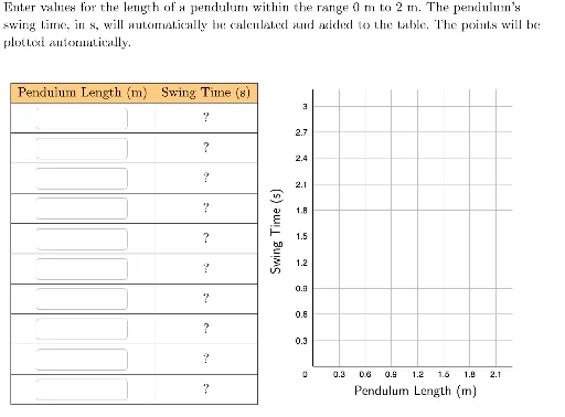
This example demonstrates the relationship between pendulum length and swing time. Key mathematical concepts include functions, trigonometry, and data fitting. Using GeoGebra commands such as Polygon, Textfield, and Zip, the trajectory of the pendulum swing can be constructed and data collected. Suitable for high school physics and mathematics courses.
GeoGebra Commands & Parameters
Polygon({(-0.4, -0.2), (-0.4, 3.2), (2.3, 3.2), (2.3, -0.2)}) → viewBoxTextfield(x1text) → boxX1Textfield(x9text) → boxX9Textfield(x8text) → boxX8Textfield(x7text) → boxX7Textfield(x6text) → boxX6Textfield(x5text) → boxX5Textfield(x4text) → boxX4Textfield(x3text) → boxX3Textfield(x2text) → boxX2Textfield(x10text) → boxX10Zip(f(A), A, xVals) → yValsZip((A, B), A, xVals, B, yVals) → pointsToPlotLaTeX("\text{Pendulum Length (m)}") → xLabelRotateText(LaTeX["\text{Swing Time (s)}"], 90°) → yLabelTableText({Join[{{"\cellcolor{#ffcc80}{\text{Pendulum Length (m)}}"}, Zip[(("\vphantom{\small\frac{1}{2}}" * A) * ""), A, xVals]}], Join[{{"\cellcolor{#ffcc80}{\text{Swing Time (s)}}"}, yVals}]}, "|_vc") → dataLaTeX("\text{Enter values for the length of a pendulum within the range \(0\) m to \(2\) m. The pendulum's\\swing time, in s, will automatically be calculated and added to the table. The points will be\\plotted automatically.}") → TEXT
AI Drawing Prompt Reference
Create a graph showing the relationship between pendulum length and swing time. Start by drawing a view box with axes, then input text fields for pendulum lengths ranging from 0 meters to 2 meters. Next, plot the function curve representing the relationship, and automatically add data points to the table and plot them.
The prompt above was compiled from the original drawing commands and is for reference only.