
Dandelin's Theorem in Stereometry
Loading the math board and drawing, please wait…
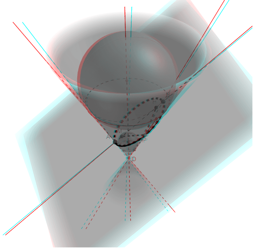
This example illustrates Dandelin's theorem, showing the relationship between the inscribed sphere and the conic section in a cone. Key mathematical concepts include cones, conic sections, and solid geometry. Using GeoGebra commands such as ConeInfinite, Rotate, and IntersectPath, the geometric meaning of the theorem is intuitively understood. Suitable for high school solid geometry courses.
GeoGebra Commands & Parameters
ConeInfinite((0, 0, 0), zAxis, α) → aAxes(a) → d, e, fRotate(f, (-α), yAxis) → f'_1Point(f'_1) → ARotate(f, α, yAxis) → f'Point(f') → BPlane(A, B_1, B) → bIntersectPath(b, a) → cAxes(c) → i, jAngularBisector(f', i) → b2, b1Center(a) → OVector(O, B) → vOBAngle(Vector[A, B], Vector[A, O]) → βVector(O, A) → vOARotate(vOA, β / 2, A, k) → vOA'Angle(Vector[B, A], Vector[O, B]) → α1Rotate(vOB, α1 / 2, B, k) → vOB'Ray(B, B') → gIntersect(f, b1) → GOrthogonalLine(G, i, k) → hIntersect(i, h) → HCircle(G, H, k) → pSphere(G, H) → lRay(A, A') → mIntersect(f, b2) → LOrthogonalLine(L, i, k) → nIntersect(i, n) → MCircle(L, M, k) → sPoint(c) → PLine(O, P) → a_1Segment(M, P) → b_1Segment(P, H) → e_1Sphere(L, M) → l'OrthogonalLine(L, f'_1, k) → qOrthogonalLine(G, f'_1, k) → rIntersect(f'_1, r) → CIntersect(q, f'_1) → DCircle(f, C) → tCircle(f, D) → c_1Line(O, P) → d_1Intersect(d_1, c_1) → E,Intersect(d_1, t) → F,Segment(P, F) → f_1Segment(E, P) → g_1Segment(O, E) → h_1