
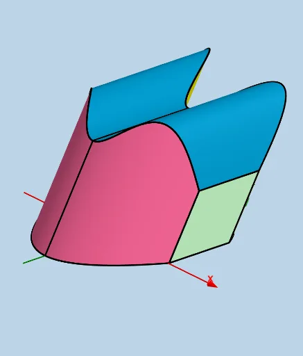
Custom Solid: Adjustable Rhombus Cross Sections Parallel to yAxis
Loading the math board and drawing, please wait…
This example demonstrates a customizable solid where cross-sections parallel to the yAxis are adjustable rhombuses with one side equal to upper(x) - lower(x). It involves core mathematical concepts such as functions, coordinate geometry, and solid geometry. The construction utilizes GeoGebra commands and objects like Intersect, Line, Segment, Rotate, Translate, Midpoint, Sphere, Textfield, Polygon, CurveCartesian, Surface, and Angle. It is suitable for high school and above students to learn about the relationship between function graphs and solid geometry, as well as how to adjust graphic properties through parameters.
GeoGebra Commands & Parameters
Intersect(lower, h, (0, -8)) → CLine(C, C + (1, 0, 0)) → cIntersect(upper, h, (0, 4)) → BSegment(C, B) → qIntersect(upper, q, (0, 4)) → GRotate(G, (ANG * pi / 180), C, c) → G'_1Translate(G'_1, Vector[C, G]) → J_1Segment(H, I) → s_1Midpoint(s_1) → A_1Segment(J, K) → q_1Midpoint(q_1) → ZMidpoint(s_1) → EMidpoint(q_1) → FMidpoint(C, G) → TLine(B, D) → iSphere(B, d) → eSegment(C, B) → pTextfield(upper) → InputBox1Textfield(lower) → InputBox2Textfield(a) → InputBox3Textfield(b) → InputBox4Segment(C, G) → k_1Line(C, G) → jSphere(G, T) → kLine(T, T + (1, 0, 0)) → mRotate(G, pi / 3, F_1, m) → G'Rotate(G', pi / 3, F_1, Line[F_1, F_1 + (1, 0, 0)]) → G''Line(F_1, F_1 + (1, 0, 0)) → nRotate(G'', pi / 3, F_1, n) → G'''Rotate(G''', pi / 3, F_1, n) → G_1Polygon(C, G, J_1, G'_1) → poly1, g_1, m_1, r_1, a_1Line(Z, Z + (1, 0, 0)) → fLine(D_1, D_1 + (1, 0, 0)) → gRotate(J, pi / 3, D_1, g) → J'Rotate(J', pi / 3, D_1, g) → J''Rotate(J'', pi / 3, D_1, g) → J'''Rotate(J''', pi / 3, D_1, g) → E_1Line(H_1, H_1 - (1, 0, 0)) → l_1Rotate(I, pi / 3, H_1, l_1) → I'Rotate(I', pi / 3, H_1, l_1) → I''Rotate(I'', pi / 3, H_1, l_1) → I'''Rotate(I''', pi / 3, H_1, l_1) → I_1Segment(G, J_1) → lSegment(J_1, G'_1) → rSegment(G'_1, C) → sLine(K, K + (1, 0, 0)) → tRotate(J, (ANG * pi / 180), K, t) → J'_1Translate(J'_1, Vector[K, J]) → K_1Polygon(K, J, K_1, J'_1) → q1, k_3, j_1, k_4, j'_1Line(I, I + (1, 0, 0)) → f_1Rotate(H, (ANG * pi / 180), I, f_1) → H'Translate(H', Vector[I, H]) → H''Segment(H, H'') → i_1Segment(H'', H') → n_1Segment(H', I) → p_1Polygon(I, H, H'', H') → q2, i_2, h_2, h'', h'Segment(J, K_1) → b_1Segment(K_1, J'_1) → c_1Intersect(t, q_1) → L_1Segment(J'_1, L_1) → d_1CurveCartesian(t, lower(t) + ((upper(t) - lower(t)) * cos((ANG * pi / 180))), ((upper(t) - lower(t)) * sin((ANG * pi / 180))), t, a, b) → oCurveCartesian(t, upper(t) + ((upper(t) - lower(t)) * cos((ANG * pi / 180))), ((upper(t) - lower(t)) * sin((ANG * pi / 180))), t, a, b) → uSurface(u, lower(u) + (((upper(u) - lower(u)) * v) * cos((ANG * pi / 180))), (((upper(u) - lower(u)) * v) * sin((ANG * pi / 180))), u, a, b, v, 0, 1) → vSurface(u, lower(u) + ((upper(u) - lower(u)) * cos((ANG * pi / 180))) + (v * (upper(u) - lower(u))), ((upper(u) - lower(u)) * sin((ANG * pi / 180))), u, a, b, v, 0, 1) → wSurface(u, upper(u) + (((upper(u) - lower(u)) * v) * cos((ANG * pi / 180))), (((upper(u) - lower(u)) * v) * sin((ANG * pi / 180))), u, a, b, v, 0, 1) → e_1Angle(G, C, G'_1) → α