
Curvilinear Integral of a Scalar Field
Loading the math board and drawing, please wait…
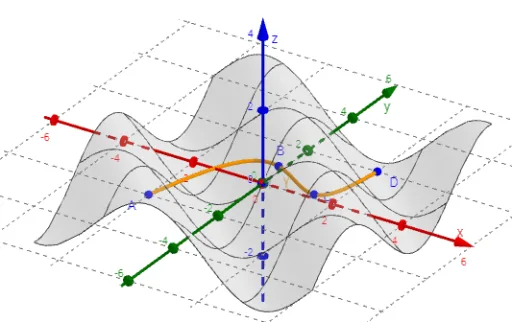
This example demonstrates the curvilinear integral of a scalar field. Using commands like Spline, Function, and CurveCartesian, complex curves can be constructed and their curvilinear integrals calculated. This example covers core concepts in calculus and is suitable for high school or university mathematics education.
GeoGebra Commands & Parameters
Spline({A, B, C, D}, 3) → γFunction(f, -4, 4, -4, 4) → f_1CurveCartesian(x(γ(t)), y(γ(t)), f(x(γ(t)), y(γ(t))), t, 0, 1) → aSurface(x(γ(t)), y(γ(t)), (s * f(x(γ(t)), y(γ(t)))), t, 0, 1, s, 0, 1) → bLength(γ, 0, 1) → cIntegral(ff, 0, (0.99999 * c)) → KurvIntSegment((0, 0), G) → gSurface((0.9999 * x(γ(t))), y(γ(t)), s, t, 0, 1, s, -2, 2) → e
AI Drawing Prompt Reference
Create a 3D visualization of a curvilinear integral of a scalar field. Start with a smooth cubic spline curve passing through four points in the plane, forming a path. Above this path, construct a space curve whose height is determined by a scalar function evaluated along the path. Then, generate a surface between the path and the space curve to represent the integral area, and add a vertical slicing plane to illustrate the integration process. Finally, draw a line segment from the origin to a point on the path, and include a semi-transparent auxiliary surface to enhance depth and visual clarity.
The prompt above was compiled from the original drawing commands and is for reference only.