
Cube Roots and Geometric Construction of Cubes
Loading the math board and drawing, please wait…
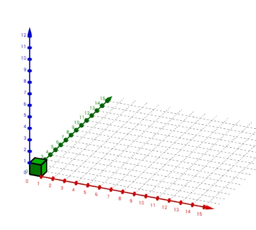
① This GeoGebra example demonstrates the geometric representation of cube roots in three-dimensional space, using a cube and its faces, edges, and vertices to visually relate cube roots to volume and side length. ② Core mathematical concepts include cube roots, properties of cubes, intersections of planes and solids, and an introduction to frequency distribution and stochastic processes, though the main focus is on the geometric construction of cube roots. ③ Construction details: The Intersect command finds intersection points, Circle and Point create basic elements, Cube constructs the solid, Sequence generates series of points (e.g., A1 to A10, B1 to B10), and multiple faces (faceABCD, faceADHE, etc.) and edges (edgeAD, edgeAB, edgeBC) are defined, with parameters A, n, B, C controlling the setup. ④ Suitable for middle school to early university students, this example helps understand the geometric meaning of cube roots and serves as an interdisciplinary teaching case combining solid geometry with statistics.
GeoGebra Commands & Parameters
Intersect(xAxis, yAxis) → ACircle(A, cbrt(n)) → cIntersect(c, xAxis, 2) → BPoint(Circle[B, Distance[A, B], Segment[A, B]]) → CCube(A, B, C) → a, D, faceCDHG, faceEFGH, edgeAD, edgeAB, edgeBC, edgeCD, edgeAE, edgeDH, edgeEH, edgeEF, E, edgeBF, edgeFG, edgeCG, edgeGH, F, G, H, faceABCD, faceADHE, faceABFE, faceBCGFSequence(Segment[A + (i * (0, 0, 1)), B + (i * (0, 0, 1))], i, 1, edgeAB) → list1Sequence(Segment[A + (i * (0, 1, 0)), E + (i * (0, 1, 0))], i, 1, edgeAB) → list2Sequence(Segment[A + (i * (1, 0, 0)), E + (i * (1, 0, 0))], i, 1, edgeAB) → list3Sequence(Segment[A + (i * (0, 1, 0)), B + (i * (0, 1, 0))], i, 1, edgeAB) → list4Sequence(Segment[A + (i * (1, 0, 0)), D + (i * (1, 0, 0))], i, 1, edgeAB) → list5Sequence(Segment[A + (i * (0, 0, 1)), D + (i * (0, 0, 1))], i, 1, edgeAB) → list6Sequence(Segment[D + (i * (0, 0, 1)), C + (i * (0, 0, 1))], i, 1, edgeAB) → list7Sequence(Segment[D + (i * (1, 0, 0)), H + (i * (1, 0, 0))], i, 1, edgeAB) → list8Sequence(Segment[B + (i * (0, 0, 1)), C + (i * (0, 0, 1))], i, 1, edgeAB) → list9Sequence(Segment[B + (i * (0, 1, 0)), F + (i * (0, 1, 0))], i, 1, edgeAB) → list10Sequence(Segment[E + (i * (0, 1, 0)), F + (i * (0, 1, 0))], i, 1, edgeAB) → list11Sequence(Segment[E + (i * (1, 0, 0)), H + (i * (1, 0, 0))], i, 1, edgeAB) → list12
AI Drawing Prompt Reference
Draw a cube in 3D space with its base centered at the origin and one base edge along the x-axis. From the origin, draw a circle with radius equal to the cube root of the cube's side length; the circle's intersection with the positive x-axis determines one vertex of the cube. Construct all edges and faces of the cube from this vertex. On each face, add equally spaced parallel line segments along the three coordinate axes, creating a grid-like pattern that covers all faces, visually relating the cube's volume to its side length and cube root.
The prompt above was compiled from the original drawing commands and is for reference only.