
Creating a Histogram with a Table
Loading the math board and drawing, please wait…
In collections
UCSS Secondary Math I Unit 4 Lesson 1
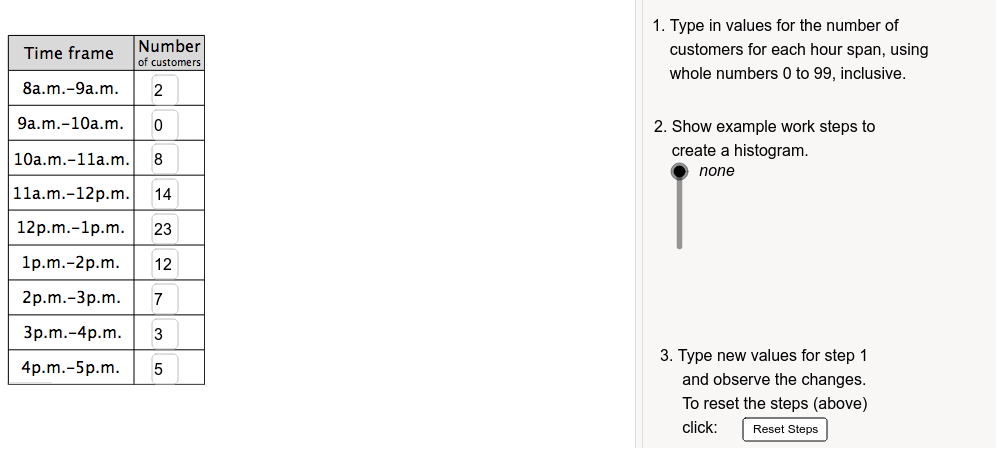
This example demonstrates how to create a histogram using tabular data. It involves core math concepts like histograms, normal distribution, linear regression, sequences and series, interest calculation, and quadrilaterals. The construction utilizes GeoGebra commands such as Textfield, Polygon, Segment, Sequence, Vector, Sort, Element, and If. It is suitable for high school mathematics education or introductory data analysis learning.
GeoGebra Commands & Parameters
Textfield(d1) → inputD1Polygon((0, 11), (If[showSteps > t0, t1, t2], 11), (If[showSteps > t0, t1, t2], 12), (0, 12)) → tableHeader, b, c, d, eSegment((0, 10), (If[showSteps > t0, t1, t2], 10)) → fSegment((0, 9), (If[showSteps > t0, t1, t2], 9)) → gSegment((0, 8), (If[showSteps > t0, t1, t2], 8)) → hSegment((0, 7), (If[showSteps > t0, t1, t2], 7)) → iSegment((0, 6), (If[showSteps > t0, t1, t2], 6)) → jSegment((0, 5), (If[showSteps > t0, t1, t2], 5)) → kSegment((0, 4), (If[showSteps > t0, t1, t2], 4)) → lSegment((0, 3), (If[showSteps > t0, t1, t2], 3)) → mSegment((t1, 0), (t1, 12)) → sTextfield(d2) → inputD2Textfield(d3) → inputD3Textfield(d4) → inputD4Textfield(d5) → inputD5Textfield(d6) → inputD6Textfield(d7) → inputD7Textfield(d8) → inputD8Segment((0, 2), (If[showSteps > t0, t1, t2], 2)) → aTextfield(d9) → inputD9Segment((3.2, 2), (3.2, 12)) → qSegment((0, 2), (0, 11)) → nSegment((If[showSteps > t0, t1, t2], 2), (If[showSteps > t0, t1, t2], 11)) → pSequence(Segment[(i, -0.3), (i, 0)], i, 7, 18) → xAxisHashMarksVector((10, 0), (18.8, 0)) → xAxisRVector((10, 0), (6.2, 0)) → xAxisLVector((7, 2), (7, -0.8)) → yAxisBSort({d1, d2, d3, d4, d5, d6, d7, d8, d9}) → orderedElement(ordered, 9) → grIf(gr < 12, 1, If[gr < 24, 2, If[gr < 30, 3, If[gr < 60, 4, 5]]]) → ySetSequence(Segment[(i, 0), (i, 12)], i, 8, 1000) → gridVSequence(Segment[(7, i), (1000, i)], i, 1, 12) → gridHVector((7, 2), (7, 12.8)) → yAxisTSequence(Segment[(6.7, i), (7, i)], i, 1, 12) → yAxisHashMarksIf(ySet ≟ 1, 1, If[ySet ≟ 2, 2, If[ySet ≟ 3, 2.5, If[ySet ≟ 4, 5, 10]]]) → scaleFactorPolygon((8, 0), (9, 0), (9, d1 / scaleFactor), (8, d1 / scaleFactor)) → hist89, t, a_1, b_1, c_1Polygon((9, 0), (10, 0), (10, d2 / scaleFactor), (9, d2 / scaleFactor)) → hist910, d_1, e_1, f_1, g_1Polygon((10, 0), (11, 0), (11, d3 / scaleFactor), (10, d3 / scaleFactor)) → hist1011, h_1, i_1, j_1, k_1Polygon((11, 0), (12, 0), (12, d4 / scaleFactor), (11, d4 / scaleFactor)) → hist1112, l_1, m_1, n_1, p_1Polygon((12, 0), (13, 0), (13, d5 / scaleFactor), (12, d5 / scaleFactor)) → hist121, q_1, r_1, s_1, t_1Polygon((13, 0), (14, 0), (14, d6 / scaleFactor), (13, d6 / scaleFactor)) → hist12, a_2, b_2, c_2, d_2Polygon((14, 0), (15, 0), (15, d7 / scaleFactor), (14, d7 / scaleFactor)) → hist23, e_2, f_2, g_2, h_2Polygon((15, 0), (16, 0), (16, d8 / scaleFactor), (15, d8 / scaleFactor)) → hist34, i_2, j_2, k_2, l_2Polygon((16, 0), (17, 0), (17, d9 / scaleFactor), (16, d9 / scaleFactor)) → hist45, m_2, n_2, p_2, q_2
AI Drawing Prompt Reference
Create a histogram with a table for input data. The histogram consists of multiple bars, each bar's height representing the input data, aligned on the horizontal axis with gaps between bars. Include axis with tick marks and a grid background to show data distribution.
The prompt above was compiled from the original drawing commands and is for reference only.