
Convergence demo of Jacobi vs Gauss-Seidel iterations for linear systems
Loading the math board and drawing, please wait…
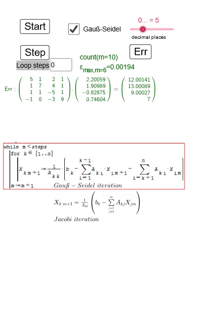
This GeoGebra example demonstrates how the Jacobi method and the Gauss-Seidel method iteratively solve a linear equation system Ax = b, showing their convergence behavior and how the error decreases across iterations. Key concepts include linear systems, iterative solvers (Jacobi / Gauss-Seidel), matrix-based update rules, an error tolerance ε, and iteration-to-iteration differences (difference & slope). The construction relies on GeoGebra commands such as If (conditional stopping when the error threshold is met), Sequence and Flatten (building and restructuring the iteration sequence), and Textfield (displaying iteration results and error estimates). Objects like X0 and the stacked iterates X_{00}…X_{08} (together with X_O, X_{01}…X_{07}) store successive vectors, while variables and modules such as JAC/JS/StepJS and GSR/GSL/GS/GSX/StepGS organize the two iteration schemes. Interactive controls (button1/button2/button3) and looping structures (Loop, InputBox1) allow users to run the iteration step-by-step, and error indicators (GSErr, txtErr, ε) visualize convergence in a clear, hands-on way. Suitable for high school advanced study and undergraduate courses in linear algebra and numerical analysis.
GeoGebra Commands & Parameters
Length(A) → nIf(k < n, "-Sum(Element(A, " + k + ", i) * Element(X_{" + (If[m < 10, O + m, "" + m]) + "}, i), i, " + (k + 1) + ", n)", "-0") → GSRIf(k > 1, "-Sum(Element(A, " + k + ", i) * Element(X_{" + (If[m < 9, O + (m + 1), "" + (m + 1)]) + "}, i), i, 1, " + (k - 1) + ")", "-0") → GSLSequence("Delete(X_{" + (If[j < 10, O + (j), "" + (j)]) + "}" + ")", j, 1, m) → GSdelFlatten({"X_{" + (If[m < 9, O + (m + 1), "" + (m + 1)]) + "}=" + GSX, Sequence[{"SetValue(k," + (j) + ")", GS}, j, 1, n], "SetValue(m," + (m + 1) + ")"}) → StepGSFlatten({"X_{" + (If[m < 9, O + (m + 1), "" + (m + 1)]) + "}=" + GSX, Sequence[{"SetValue(k," + (j) + ")", JS}, j, 1, n], "SetValue(m," + (m + 1) + ")"}) → StepJSTextfield(Loop) → InputBox1Sequence(X_O, j, 1, n) → X_{00}
AI Drawing Prompt Reference
Draw a diagram showing the convergence of iterative methods for solving a linear system. Include a 2D coordinate plane with axes for two unknowns. From an initial point, draw two colored polyline paths, one for Jacobi iteration and one for Gauss-Seidel iteration, each consisting of discrete points connected by segments, converging toward the intersection point of two lines (the exact solution). Mark an error tolerance threshold; stop when the distance from the current point to the solution is below it. Include an input box for iteration count and three buttons for step, run, and reset. Display current iteration number and error value near the plot, with error decreasing over iterations.
The prompt above was compiled from the original drawing commands and is for reference only.