Demonstrating Pick’s Theorem for Lattice Polygons

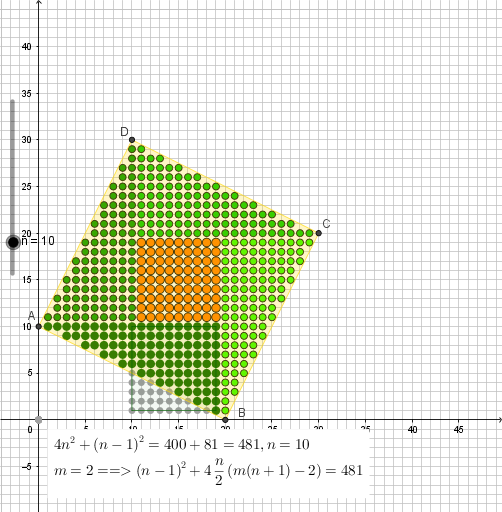
This GeoGebra example builds a simple lattice polygon on a coordinate grid and labels its boundary and interior lattice points so you can visually verify Pick’s Theorem. It demonstrates the key idea that the polygon’s area can be computed from the number of lattice points on the boundary (B) and strictly inside the polygon (I). The core concepts include lattice points (integer-coordinate points), simple polygons, and the relation Area = I + B/2 − 1 (as implemented via the constructed objects). Construction-wise, the example uses GeoGebra commands Polygon and Flatten to form the polygon and to manage/flatten the generated point lists. It also introduces supporting parameters and named objects (e.g., Pick, B, I1, and several auxiliary quantities) to connect the geometric figure with the counting variables needed for the theorem. Suitable for advanced high school learners, math competition preparation, and early university discrete geometry/number theory instruction.