
Constructing Graphs of Derivative Functions (Intuitively)
Loading the math board and drawing, please wait…
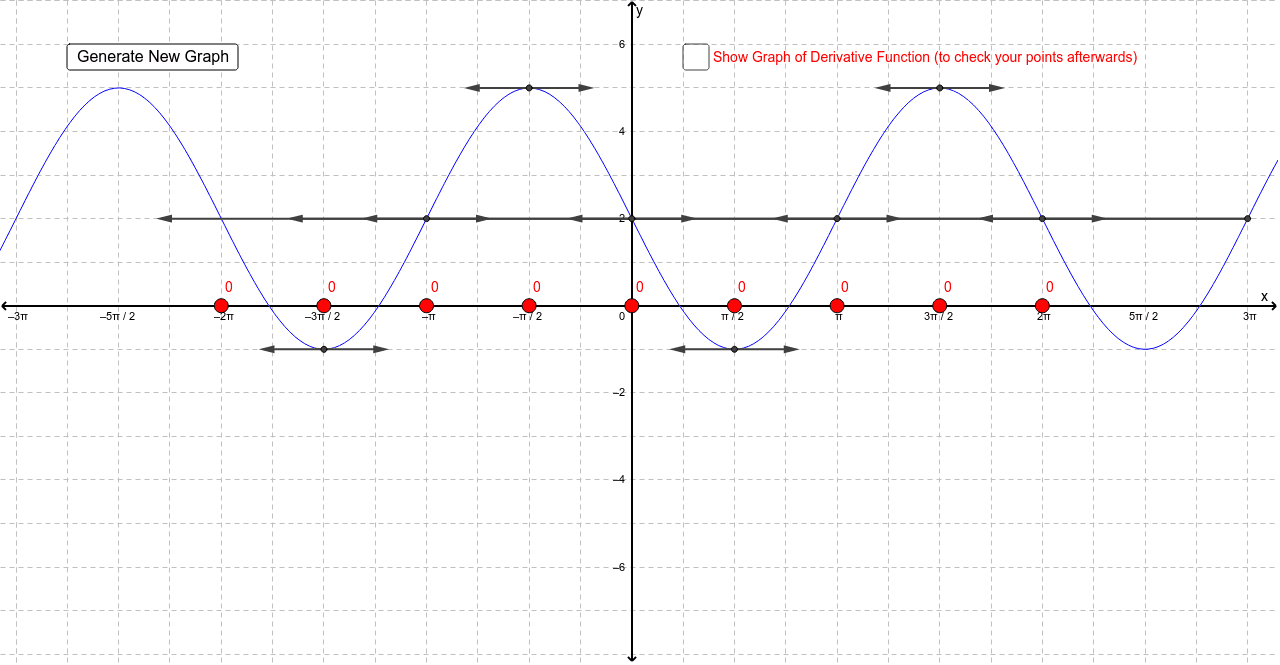
This example demonstrates how to intuitively understand the construction of derivative function graphs by moving points. Core math concepts include derivatives, function graphs, upper and lower sums or Riemann sums, and tangent functions. Construction highlights using GeoGebra commands/objects from the summary: Random, RandomElement, Point, Circle, Intersect, Vector; objects: list1, f, b, c, d, a, g, vert_A, A, line_A, circle_A, A_2, A_3, A_1, u_A, v_A, vert_B, B, circle_B, line_B, B_1, B_2, B_3, u_B, v_B, vert_C, C, C_1, circle_C, line_C, C_2, C_3, u_C, v_C, vert_D, D, line_D, circle_D, D_1, D_2. Suitable for high school or introductory calculus students.
GeoGebra Commands & Parameters
Random(1, 2) → bRandom(-3, 3) → cRandom(-3, 3) → dRandomElement(list1) → aPoint(vert_A) → ACircle((x(A), g(x(A))), 1) → circle_AIntersect(circle_A, line_A, 1) → A_2Intersect(circle_A, line_A, 2) → A_3Intersect(g, vert_A, (0, 1)) → A_1Vector(A_1, A_3) → u_AVector(A_1, A_2) → v_APoint(vert_B) → BCircle((x(B), g(x(B))), 1) → circle_BIntersect(g, vert_B, (1.5707963267948966, 3.5)) → B_1Intersect(circle_B, line_B, 1) → B_2Intersect(circle_B, line_B, 2) → B_3Vector(B_1, B_2) → u_BVector(B_1, B_3) → v_BPoint(vert_C) → CIntersect(g, vert_C, (3.141592653589793, 1)) → C_1Circle((x(C), g(x(C))), 1) → circle_CIntersect(circle_C, line_C, 1) → C_2Intersect(circle_C, line_C, 2) → C_3Vector(C_1, C_3) → u_CVector(C_1, C_2) → v_CPoint(vert_D) → DCircle((x(D), g(x(D))), 1) → circle_DIntersect(g, vert_D, (4.71238898038469, -1.5)) → D_1Intersect(circle_D, line_D, 1) → D_2Intersect(circle_D, line_D, 2) → D_3Vector(D_1, D_2) → u_DVector(D_1, D_3) → v_DPoint(vert_E) → ECircle((x(E), g(x(E))), 1) → circle_EIntersect(g, vert_E, (6.283185307179586, 1)) → E_1Intersect(circle_E, line_E, 1) → E_2Intersect(circle_E, line_E, 2) → E_3Vector(E_1, E_2) → u_EVector(E_1, E_3) → v_EPoint(vert_F) → FCircle((x(F), g(x(F))), 1) → circle_FIntersect(g, vert_F, (-1.5707963267948966, -1.5)) → F_1Intersect(circle_F, line_F, 1) → F_3Intersect(circle_F, line_F, 2) → F_2Vector(F_1, F_3) → u_FVector(F_1, F_2) → v_FPoint(vert_G) → GCircle((x(G), g(x(G))), 1) → circle_GIntersect(g, line_G, (-3.141592653589793, 1)) → G_1Intersect(circle_G, line_G, 1) → G_2Intersect(circle_G, line_G, 2) → G_3Vector(G_1, G_2) → u_GVector(G_1, G_3) → v_GPoint(vert_H) → HCircle((x(H), g(x(H))), 1) → circle_HIntersect(g, line_H, (-4.71238898038469, 3.5)) → H_1Intersect(circle_H, line_H, 1) → H_2Intersect(circle_H, line_H, 2) → H_3Vector(H_1, H_2) → u_HVector(H_1, H_3) → v_HPoint(vert_I) → ICircle((x(I), g(x(I))), 1) → circle_IIntersect(circle_I, line_I, 1) → I_2Intersect(circle_I, line_I, 2) → I_3Intersect(g, line_I, (-7.853981633974411, -2)) → I_1Vector(I_1, I_2) → u_IVector(I_1, I_3) → v_I
AI Drawing Prompt Reference
Draw a function graph and its derivative graph, intuitively demonstrating the concept of derivatives by randomly selecting points and drawing circles and line segments. For each point on the function graph, draw a circle and find its intersections with the function. Connect these intersection points to form line segments that approximate tangents. Use these line segments and circles to show the local rate of change of the function, thereby intuitively understanding the geometric meaning of derivatives.
The prompt above was compiled from the original drawing commands and is for reference only.