
Constant Multiple Derivative Rule
Loading the math board and drawing, please wait…
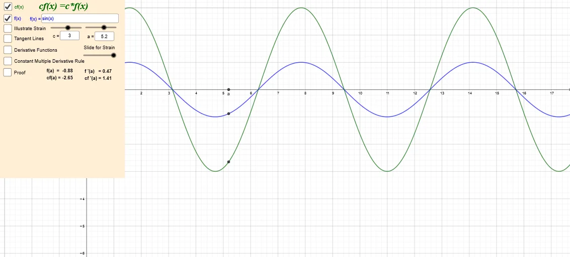
This example demonstrates the constant multiple derivative rule in function graphs. The key mathematical concepts involve derivatives, function transformations, and geometric construction. Construction involves using GeoGebra commands such as Textfield, Vector, InputBox, etc. to create function images and label key points. Suitable for high school or undergraduate students to understand derivative concepts and function properties.
GeoGebra Commands & Parameters
Textfield(f) → InputBox1Textfield(a) → InputBox3Textfield(c) → InputBox2Vector(A, B) → uVector((a, 0), (a, (sgn(c) * f(a)) + (e * (cf(a) - (sgn(c) * f(a)))))) → vVector((a, f(a)), (a + 1, f(a))) → wVector((a, cf(a)), (a + 1, cf(a))) → iVector((a + 1, f(a)), (a + 1, t_{1}(a + 1))) → jVector((a + 1, cf(a)), (a + 1, t_{2}(a + 1))) → mVector((a, 0), (a, f'(a))) → pVector((a, 0), (a, cf'(a))) → q
AI Drawing Prompt Reference
Draw a function graph illustrating the constant multiple derivative rule. Include the original function f(x), its derivative f'(x), and the constant multiple function cf(x). Use arrows and labels to mark key points, such as the value of f(x) at x=a, the value of f'(x) at x=a, and the value of cf(x) at x=a. Arrows indicate changes in function values and the meaning of derivatives. Labels help identify these key points. The image should clearly show these relationships to help understand the derivative rule.
The prompt above was compiled from the original drawing commands and is for reference only.