Connectivity Matrix: Visualizing Vertex Links in a Tetrahedron

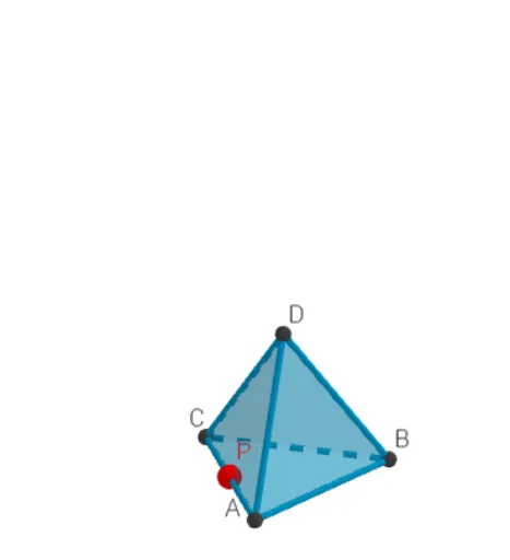
This GeoGebra example demonstrates a connectivity matrix (adjacency matrix) for a tetrahedron, visually mapping which vertices are connected by edges. The core mathematical concept is graph theory's adjacency matrix, applied to the six edges of a tetrahedron, combined with solid geometry of vertices, edges, and faces. Construction highlights: the Tetrahedron command creates the solid; vertices A, B, C, D and edges RibbeAB, RibbeAC, etc. are defined; TableText generates the matrix table; Circle, Intersect, Rotate, and Point assist in labeling and rotating the view; objects like rijA, rijB store matrix rows, while MM and n handle matrix operations. Suitable for high school or university students learning solid geometry, introductory graph theory, or matrix applications, and useful for demonstrating network connectivity in mathematical modeling.