Visualizing the Connectivity Matrix of a Cube

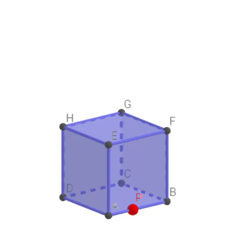
This GeoGebra example constructs a cube and generates a connectivity matrix using TableText, visually representing the adjacency relationships among the cube's vertices. The core mathematical concepts include graph theory (adjacency matrix) and solid geometry (vertices, edges, faces of a cube). The construction uses commands such as Circle, Intersect, Rotate, Cube, TableText, and Point, with objects including vertices A through H, face polygons (zijvlakABCD, etc.), edges (RibbeAD, etc.), and lists (lijstA to lijstH) that store vertex data. The matrix is displayed as a table, making the connectivity explicit. This example is suitable for high school or early college students, serving as a visual aid for understanding graph representations and their geometric interpretations, and can be used in mathematics or computer science courses.