
Confidence Intervals for Population Proportion Construction
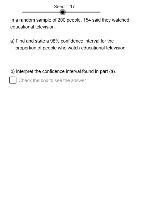
Loading the math board and drawing, please wait…
This example demonstrates how to construct and visualize confidence intervals for population proportions. Key mathematical concepts include: point estimation (sample proportion p-hat), confidence interval formula, principle of interval estimation, and relationship between significance level α and confidence level. Construction details: Use Sequence command to generate multiple sample sequences and Element command to extract sample proportions; calculate upper bound UB and lower bound LB using Z-critical value (ZCrt) and standard error (StEr); dynamically display confidence interval graphics through Cnf and CnfDc objects; use slider animation to adjust confidence level and sample size, intuitively observing interval width changes. Suitable for high school statistics teaching or introductory college statistics courses, helping students understand the statistical meaning of confidence intervals and their influencing factors.
GeoGebra Commands & Parameters
Sequence(Mod[4 + (13 * k), 32] + 20, k, 1, 32) → OpSq, {37, 50, 31, 44, 25, 38, 51, 32, 45, 26, 39, 20, 33, 46, 27, 40, 21, 34, 47, 28, 41, 22, 35, 48, 29, 42, 23, 36, 49, 30, 43, 24}Element(OpSq, Seed) → NmCh1Element(CnfSq, Ch2) → CnfElement(XSq, Ch1) → XElement(NSq, Ch1) → NElement(OpSq, Seed) → OptElement(DDSq, Ch1) → DD0