
Confidence Interval Variation Problems
Loading the math board and drawing, please wait…
In collections
Statistics Demonstrations
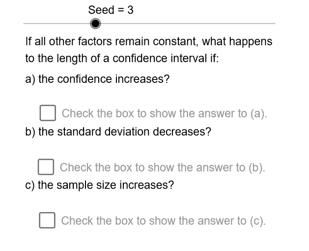
This example demonstrates how a confidence interval changes when the confidence level, standard deviation, or sample size varies. Key math concepts include confidence intervals, standard deviation, sample size, and statistics. It is constructed using GeoGebra commands like Sequence, Element, and If, making it suitable for high school students and beginners in statistics.
GeoGebra Commands & Parameters
Sequence(Mod[(3 * k), 8], k, 0, 7) → RndSqElement(RndSq, Seed) → QstIf(Mod[Qst - 1, 2] ≟ 0, 0, 1) → AIf(Mod[Qst - 1, 4] > 1, 1, 0) → BIf(Qst - 1 > 3, 1, 0) → CIf(A ≟ 1, Ainc, Adec) → PartAIf(B ≟ 1, Binc, Bdec) → PartBIf(C ≟ 1, Cinc, Cdec) → PartCIf(A ≟ 1, "increases.", "decreases.") → DirAIf(B ≟ 1, "increases.", "decreases.") → DirBIf(C ≟ 1, "decreases.", "increases.") → DirC
AI Drawing Prompt Reference
Create a statistical graph showing three key objects representing how a confidence interval changes with confidence level, standard deviation, and sample size variations. Use sliders to control these variables and observe the corresponding increase or decrease in the objects. Indicate the direction of change (increase or decrease) with arrows. First draw the three base objects, then modify their appearance based on slider values, and finally connect them to form a cohesive graph.
The prompt above was compiled from the original drawing commands and is for reference only.