
Composite Transformations of Tangent Function and Stochastic Curve Sketching
Loading the math board and drawing, please wait…
In collections
Mapping Diagrams: From AB to C&DE, Resource
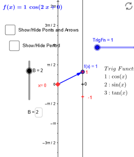
This example demonstrates the graphical behavior of the tangent function under composite transformations, combined with stochastic process concepts to illustrate dynamic curve sketching. Core mathematical concepts include periodicity, asymptotes, reflection, means (averages), and stochastic or random processes. Construction highlights: using GeoGebra commands such as Element, Point, Vector, Segment, Sequence, Textfield, Derivative, and Zip, with objects like B, C, TrigFn, k, A, TrigL, f, a_1, a, f_a, u, text1, text2, x_0, f_x, etc. Parameters are controlled via sliders or text inputs, derivatives are used to analyze function changes, and sequences generate random points or curves. Suitable for high school to undergraduate mathematics education, useful for understanding trigonometric transformations, function graphing, and visualization of stochastic processes.
GeoGebra Commands & Parameters
Element(TrigL, TrigFn) → fPoint(yAxis) → aVector(a, f_a) → uSegment(C_1, D) → eVector(E, F) → vSequence((k, f(k)), k, C - π, C + π, 0.5235987755982988) → list1Sequence(Vector[(0, k), (2, f(k))], k, C - π, C + π, 0.5235987755982988) → list2Sequence(Segment[(i, f(i)), ((2 * C) - i, f((2 * C) - i))], i, C - π, C, 0.5235987755982988) → list3Vector(G, H) → wSegment(f_x, J) → jSequence(Segment[(i, f(i)), (π - i, f(π - i))], i, 0, 3.141592653589793, 0.5235987755982988) → suplTextfield(B) → inputBox1Textfield(C) → InputBox1Derivative(f) → f'Vector(f_a, (2, y(f_a) + f'(y(a)))) → hSequence(-5, 5) → nlistZip(((1 / B * ((2 * k) + 1)) * π / 2) - C / B, k, nlist) → xtrslistZip((z, f(z)), z, xtrslist) → xtrsptsZip(((1 / B * k) * π) - C / B, k, nlist) → xrtclistZip((z, f(z)), z, xrtclist) → xtrcptsTextfield(A) → InputBox2Segment(a, Q) → lSegment(a, P) → mVector(P, f_a) → nVector(Q, f_a) → pSegment(f_x, M) → sSegment(f_x, R) → q