Complex Square Mapping Between Two Planes

Loading the math board and drawing, please wait…

2018-05-01 02:08

In collections Mapping Diagrams to Visualize Complex Analysis

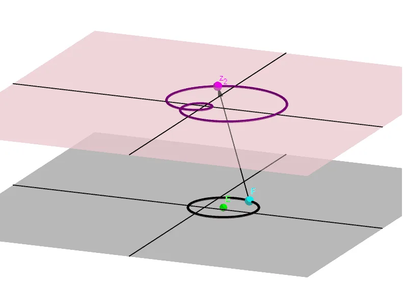
This example demonstrates the geometric representation of a complex square mapping between two planes, visually illustrating the mapping relationship through dynamic graphics. The core mathematical concepts involved include complex numbers, plane mappings, geometric transformations, and loci. The construction highlights GeoGebra commands and objects such as Point, OrthogonalPlane, Line, Translate, OrthogonalLine, Circle, Locus, and Vector. It is suitable for high school and above learners to understand the geometric meaning and dynamic changes of complex mappings.

GeoGebra Commands & Parameters

Point(zAxis) → I
OrthogonalPlane(I, zAxis) → b
Point(xAxis) → A
Point(xAxis) → B
Line(A, B) → f
Point(yAxis) → C
Point(yAxis) → D
Line(C, D) → g
Translate(f, Vector[I]) → f'
Translate(g, Vector[I]) → g'
OrthogonalLine(E, xOyPlane) → h
Circle(E, 1, h) → c
Point(c) → F
Translate(z_1, Vector[I]) → z_2
Locus(z_2, F) → loc1
Vector(F, z_2) → u

AI Drawing Prompt Reference

Draw a complex square mapping from one plane to another. Start by taking point I on the z-axis and constructing a plane b perpendicular to the z-axis through I. Take points A and B on the x-axis and connect them to form line f. Take points C and D on the y-axis and connect them to form line g. Translate lines f and g along vector I to get f' and g'. On the xOy plane, take point E and construct a line h perpendicular to the xOy plane through E. Draw a circle c with radius 1 centered at E. Take point F on circle c and translate F along vector I to get point z_2. The trajectory of F and z_2 forms a locus curve loc1.

The prompt above was compiled from the original drawing commands and is for reference only.