
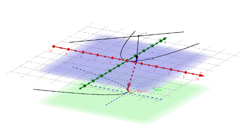
Complex Linear Mapping Diagram f(z) = Bz; Parametric Curve
Loading the math board and drawing, please wait…
This example demonstrates the effect of the complex linear mapping f(z) = Bz on a parametric curve, involving core concepts like complex numbers, linear transformations, parametric equations, and complex plane mappings. It utilizes GeoGebra commands such as Sequence, Zip, Textfield, Vector, CurveCartesian, Intersect, Point, Circle, ToPolar, and Locus to visually reveal the transformation properties, making it suitable for high school and above learners to understand the intuitive representation of complex function transformations and geometric mappings.
GeoGebra Commands & Parameters
Sequence(t + ((Ax * t^(2)) * ί), t, -3, 3, 0.5) → z_*Zip((x(z), y(z), height_{image}), z, fz_*) → fpoint_*Textfield(fz_*) → inputBox1Vector(z_#, f_{(z#).}) → wTextfield(f_{(z#)}) → inputBox2CurveCartesian(t, 0, height_{image}, t, -5, 5) → XhCurveCartesian(0, t, height_{image}, t, -5, 5) → YhTextfield(z_*) → inputBox3Sequence(Line[Element[z_*, j], Element[fpoint_*, j]], j, 1, 12) → list1Intersect(xAxis, yAxis) → B_1Point(xAxis) → CCircle(B_1, C) → pToPolar(B) → DLocus(f_{(z#)}, t_#) → loc1Locus(a, t_#) → loc2Locus(a, t_#) → cLocus(f_{(z#).}, t_#) → loc3Locus(A_1, t_#) → loc4Vector(A_1, z_#) → uCurveCartesian(t, (Ax * t^(2)), t, -5, 5) → γZip(Vector[A, B], A, z_*, B, fpoint_*) → fvec_*