
Phantom Graph General Cubic
Loading the math board and drawing, please wait…
In collections
Phantom Graphs
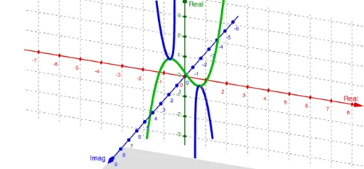
This example demonstrates the construction and properties of a phantom graph general cubic curve. It involves core mathematical concepts such as cubic polynomial functions, parametric curves, complex number roots, and coordinate geometry. Key GeoGebra commands and objects used in the construction include ComplexRoot, Plane, and CurveCartesian, as outlined in the construction summary. It is suitable for high school and above students to understand the generation and parametric characteristics of complex curves.
GeoGebra Commands & Parameters
ComplexRoot(f(x) - c) → z_1, z_2, z_3Plane((0, c, 0), (1, c, 1), (-1, c, 4)) → aCurveCartesian(t, ((-8 * A) * t^(3)) - ((2 * B) * t) + C, sqrt((3 * t^(2)) + B / A), t, -20, 20) → dCurveCartesian(t, ((-8 * A) * t^(3)) - ((2 * B) * t) + C, (-sqrt((3 * t^(2)) + B / A)), t, -20, 20) → e
AI Drawing Prompt Reference
Draw a parametric phantom graph general cubic curve, showing its generation process. First, determine three key points based on complex number roots, then construct a plane containing these points, and finally use two symmetric parametric equations to depict the shape of the cubic curve, reflecting the relationship between complex roots and coordinate geometry.
The prompt above was compiled from the original drawing commands and is for reference only.