
Lissajous Curves Demo
Loading the math board and drawing, please wait…
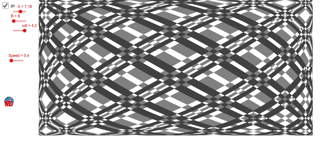
This example demonstrates the creation and manipulation of Lissajous curves, illustrating the synthesis of complex patterns from two perpendicular harmonic oscillations. Key mathematical concepts include trigonometric functions, parametric equations, complex number representation, and coordinate geometry. The construction leverages the CurveCartesian command and objects like udt, A, B, min, max, targets, velocities, sensors, and sliders to control parameters such as Speed and shape parameters a, b. It is suitable for high school and advanced learners studying function graphs, parametric equations, and complex numbers, or for mathematical modeling presentations.
GeoGebra Commands & Parameters
CurveCartesian(x(C) + (7 * sin((A * u))), y(C) + (3.5 * cos((B * u))), u, 0, (40 * π / B)) → aCurveCartesian(x(C) + (7 * cos((A * u))), y(C) + (3.5 * sin((B * u))), u, 0, (40 * π / B)) → b
AI Drawing Prompt Reference
Draw Lissajous curves resulting from the synthesis of two perpendicular harmonic oscillations. First, plot a sine curve shifted 7 units along the x-axis and a cosine curve shifted 3.5 units along the y-axis, with parameter u ranging from 0 to 40π/B. Then, plot a cosine curve shifted 7 units along the x-axis and a sine curve shifted 3.5 units along the y-axis, with parameter u also ranging from 0 to 40π/B.
The prompt above was compiled from the original drawing commands and is for reference only.