
Complex Function Mappings Visualization
Loading the math board and drawing, please wait…
In collections
complex-numbers
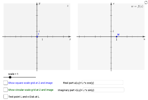
This example demonstrates how elementary complex functions transform the plane. It involves core math concepts like complex mappings, geometric transformations, and plane transformations. Constructed using GeoGebra commands like Polygon, Vector, Sequence, Textfield, and Circle. Suitable for high school and above, helping learners understand the geometric meaning and transformation properties of complex functions.
GeoGebra Commands & Parameters
Polygon((6.28, 6.28), (-6.28, 6.28), (-6.28, -6.28), (6.28, -6.28)) → q1, f, g, h, iPolygon((20.28, 6.28), (7.72, 6.28), (7.72, -6.28), (20.28, -6.28)) → q2, j, k, l, mVector((-6.5, 0), (6.5, 0)) → xaxisVector((0, -6.5), (0, 6.5)) → yaxisVector((14, -6.5), (14, 6.5)) → vaxisVector((7.5, 0), (20.5, 0)) → uaxisSequence(Segment[(k, -0.2), (k, 0.2)], k, -6, 6) → xTicksSequence(Segment[(k, -0.2), (k, 0.2)], k, 8, 20) → yTicksSequence(Segment[(-0.2, k), (0.2, k)], k, -6, 6) → uTicksSequence(Segment[(13.8, k), (14.2, k)], k, -6, 6) → vTicksSequence(CurveCartesian[x(Z) + (scale * t), y(Z) + (k * scale / 4), t, 0, 1], k, 0, 4, 1) → gridHorizontalSequence(CurveCartesian[x(Z) + (k * scale / 4), y(Z) + (t * scale), t, 0, 1], k, 0, 4, 1) → gridVerticalSequence(CurveCartesian[u(x(Z) + (scale * t), y(Z) + (k * scale / 4)) + 14, v(x(Z) + (scale * t), y(Z) + (k * scale / 4)), t, 0, 1], k, 0, 4, 1) → imagegridHorizontalSequence(CurveCartesian[u(x(Z) + (k * scale / 4), y(Z) + (t * scale)) + 14, v(x(Z) + (k * scale / 4), y(Z) + (t * scale)), t, 0, 1], k, 0, 4, 1) → imagegridVerticalSequence(CurveCartesian[x(Z) + ((scale * r) * cos(((k * 2) * π / 12))), y(Z) + ((scale * r) * sin(((k * 2) * π / 12))), r, 0, 1], k, 1, 12) → gridRaysSequence(CurveCartesian[x(Z) + ((k * scale / 4) * cos(θ)), y(Z) + ((k * scale / 4) * sin(θ)), θ, 0, (2 * π)], k, 1, 4) → gridCirclesSequence(CurveCartesian[u(x(Z) + ((k * scale / 4) * cos(θ)), y(Z) + ((k * scale / 4) * sin(θ))) + 14, v(x(Z) + ((k * scale / 4) * cos(θ)), y(Z) + ((k * scale / 4) * sin(θ))), θ, 0, (2 * π)], k, 1, 4) → imagegridCirclesTextfield(u) → InputBox1Textfield(v) → InputBox2Sequence(CurveCartesian[u(x(Z) + ((scale * r) * cos(((k * 2) * π / 12))), y(Z) + ((scale * r) * sin(((k * 2) * π / 12)))) + 14, v(x(Z) + ((scale * r) * cos(((k * 2) * π / 12))), y(Z) + ((scale * r) * sin(((k * 2) * π / 12)))), r, 0, 1], k, 1, 12) → L_1Circle(L, ε) → c
AI Drawing Prompt Reference
Create a visualization of complex function mappings with two rectangles as backgrounds, one spanning the entire canvas and the other on the right. Include coordinate axes and tick marks, and draw grid lines inside both rectangles. Display the images of functions u and v within the right rectangle, showing transformed grids with different colors. Add concentric circles and radial lines inside the left rectangle to illustrate the geometric meaning of complex functions.
The prompt above was compiled from the original drawing commands and is for reference only.