
Completing the Square: GeoGebra Geometric Visualization
Loading the math board and drawing, please wait…
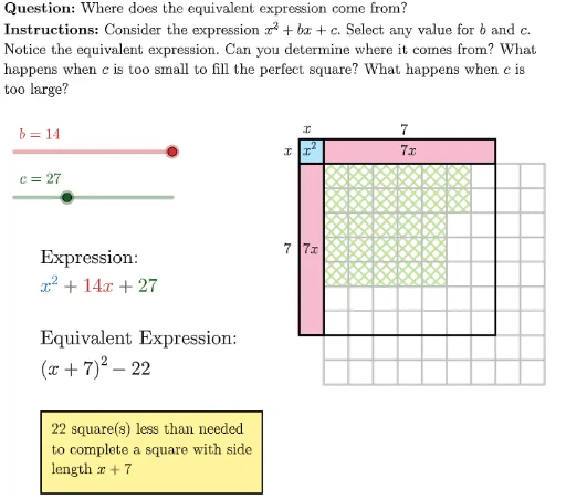
This GeoGebra example dynamically demonstrates the geometric meaning of completing the square, transforming abstract algebraic operations into intuitive area-filling problems. Core mathematical concepts include the perfect square formula, conversion between general form and vertex form of quadratic equations, and geometric interpretation of completing the square. Construction details: Uses LaTeX commands to dynamically display algebraic expression evolution, Polygon to draw squares and rectangles visualizing the 'completing' operation, Sequence to generate horizontal and vertical grid lines, with objects A1, A2, A3 building step-by-step demonstration flow, combined with interactive elements like TryAnother and Initialize for personalized practice. Suitable for middle school students (grade 8+) learning completing the square, or as a teaching aid for teachers demonstrating quadratic equation solution techniques.
GeoGebra Commands & Parameters
LaTeX((((("\text{" * QUESTION) * "\\") * INSTRUCTIONS) * "}")) → TEXTLaTeX(("b=" * b)) → bLabelLaTeX(("c=" * c)) → cLabelSequence(Segment[Point[{1, j}], Point[{10, j}]], j, -10, -1) → horizontalLinesSequence(Segment[Point[{k, -1}], Point[{k, -10}]], k, 1, 10) → verticalLinesPolygon({(0, 0), (1, 0), (1, -1), (0, -1)}) → A1Polygon((1, -1 - floorRootC), (1 + floorRootC, -1 - floorRootC), 4) → A4aPolygon({(0, 0), (1, 0), (1, -1), (0, -1)}) → A1borderPolygon({(1, 0), (1 + halfB, 0), (1 + halfB, -1), (1, -1)}) → A2Polygon({(1, 0), (1 + halfB, 0), (1 + halfB, -1), (1, -1)}) → A2borderPolygon({(0, -1), (1, -1), (1, -1 - halfB), (0, -1 - halfB)}) → A3Polygon({(0, -1), (1, -1), (1, -1 - halfB), (0, -1 - halfB)}) → A3borderPolygon({(1 + floorRootC, -1), (1 + floorRootC + 1, -1), (1 + floorRootC + 1, -1 - Min[leftOverC, floorRootC]), (1 + floorRootC, -1 - Min[leftOverC, floorRootC])}) → A4bPolygon({(1, -1 - floorRootC), (1, -1 - floorRootC - 1), (1 + Max[leftOverC - floorRootC, 0], -1 - floorRootC - 1), (1 + Max[leftOverC - floorRootC, 0], -1 - floorRootC)}) → A4cPolygon({(0, 0), (halfB + 1, 0), (halfB + 1, (-(halfB + 1))), (0, (-(halfB + 1)))}) → fullSquareText("x^2", (0, 0), true, true) → labelAText((("\vphantom{x^2}" * If[halfB ≟ 1, "", "" + halfB]) * "x"), (1 + (halfB - 1) / 2, 0), true, true) → labelBText((("\vphantom{x^2}" * If[halfB ≟ 1, "", "" + halfB]) * "x"), (0, -1 - (halfB - 1) / 2), true, true) → labelCText("x", (0, 0.75), true, true) → labelDText(halfB, (1 + (halfB - 1) / 2, 0.75), true, true) → labelEText("\vphantom{x^2}x", (-0.75, 0), true, true) → labelFText(("\vphantom{x^2}" * halfB), (-0.75, -1 - (halfB - 1) / 2), true, true) → labelG
AI Drawing Prompt Reference
Draw a 10 by 10 grid with horizontal lines from y = -10 to -1 and vertical lines from x = 1 to 10. Place a unit square at the origin to represent x², attach a rectangle of width b/2 to its right and another of height b/2 below it for the (b/2)x terms. Add further small rectangles in the lower‑right corner to account for the constant c, completing a larger square of side 1 + b/2. Label the unit square with x², the two rectangles with (b/2)x, the outer edges with x, and show the numeric values of b/2 and c, illustrating the geometric completion of the square.
The prompt above was compiled from the original drawing commands and is for reference only.