
Comparing Normal Distributions
Loading the math board and drawing, please wait…
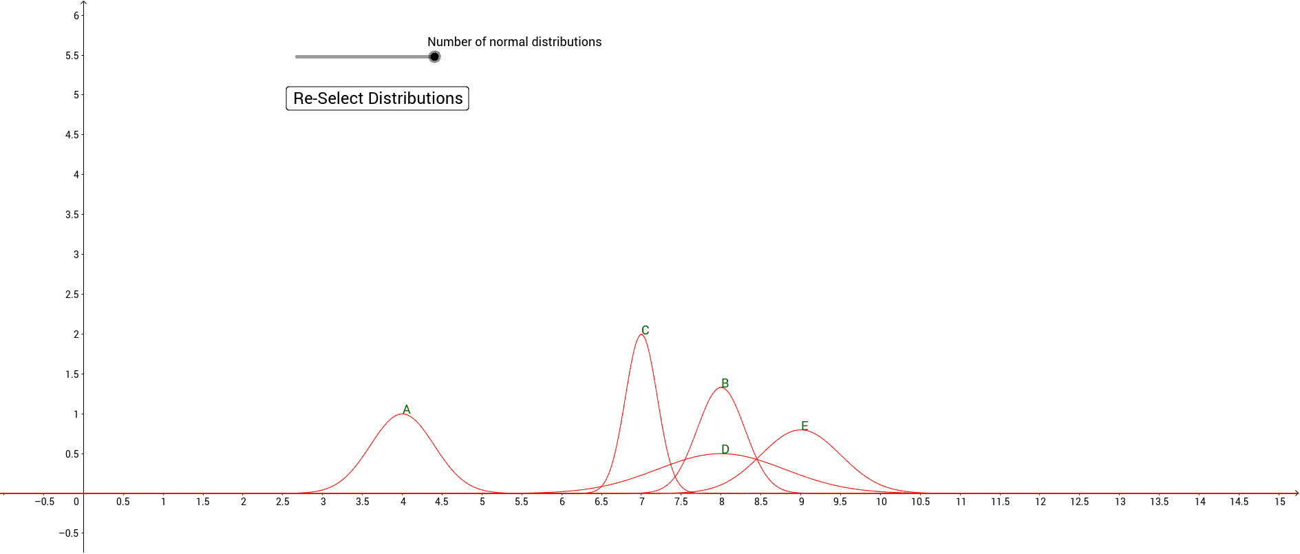
This example demonstrates how to compare two normal distributions through graphical methods, involving core math concepts like normal distributions, similarity transformations, incircles, Pythagorean theorem, random variables, and conditional probability. It utilizes GeoGebra commands such as Normal, Sequence, and Union to construct the visualizations, making it suitable for high school and above students learning probability & statistics and distribution properties.
GeoGebra Commands & Parameters
Normal(0, 1, 10) → aSequence(Random[0, 10], i, 0, n) → s1Union(Sequence[Random[1, 10] / 10, i, 1, 20], {}) → ssSequence(Random[0, 2], i, 0, n) → s2Sequence(Random[0, 10], i, 0, n) → msSequence((1 / ((Element[ss, i] * sqrt((2 * π)))) * ℯ^((-((x - Element[ms, i])^(2) / ((2 * Element[ss, i]^(2))))))), i, 1, n + 1) → s3Sequence(Text[Element[letters, i], Point[{Element[ms, i], y(Intersect[Element[s3, i], x = Element[ms, i], (10, 0.9973557010035817)])}]], i, 1, n + 1) → t