
Comparing Boxplots: Visual Analysis of Multiple Data Distributions
Loading the math board and drawing, please wait…
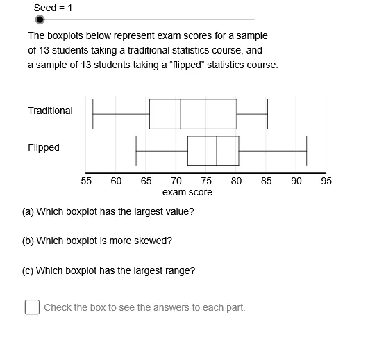
① This example demonstrates how to create and compare multiple boxplots side by side, revealing the distribution of different data groups including medians, interquartile ranges, and potential outliers. ② The core mathematical concepts involve descriptive statistics: the five-number summary (minimum, first quartile, median, third quartile, maximum), and the comparison of distributions to assess central tendency, spread, and skewness. ③ Construction highlights: using GeoGebra commands such as Sequence, Element, Max, Min, If, Segment, Mod, Text, Q1, Median, Q3, Length, and KeepIf, along with numerous objects (GrLv, GrRt, GrLf, K1–K12, DtA1, DtA2, etc.), the applet dynamically generates boxplots, often controlled by sliders or a random seed to explore variability. ④ This resource is ideal for high school or introductory college statistics courses, serving as an interactive teaching tool for comparing data distributions, understanding quartiles, and identifying outliers in real-time.
GeoGebra Commands & Parameters
Sequence(Mod[5 + (17 * k), 48] + 60, k, 0, 47) → OpSq, {65, 82, 99, 68, 85, 102, 71, 88, 105, 74, 91, 60, 77, 94, 63, 80, 97, 66, 83, 100, 69, 86, 103, 72, 89, 106, 75, 92, 61, 78, 95, 64, 81, 98, 67, 84, 101, 70, 87, 104, 73, 90, 107, 76, 93, 62, 79, 96}Element(OpSq, Seed) → OpNm1Element(DtASq, Ch4) → DtA0Max(DtA0) → AMxMin(DtA0) → AMnElement(DtBSq, Ch4) → DtB0Min(DtB0) → BMnMax(DtB0) → BMxIf((5 * LBScl) ≤ UBScl, (5 * LBScl), If[(2 * LBScl) ≤ UBScl, (2 * LBScl), LBScl]) → SclElement(AcSq, Ch4) → AccSegment(LfEP, RtEP) → nmblnElement(GrpASq, Ch4) → GrpAElement(GrpBSq, Ch4) → GrpBElement(DDSq, Ch4) → DD0Element(LblSq, Ch4) → DtLbElement(QsSqSq, Mod[Seed, 6] + 1) → QsNmSqElement(QsSq, Element[QsNmSq, 1]) → QAElement(QsSq, Element[QsNmSq, 2]) → QBElement(QsSq, Element[QsNmSq, 3]) → QCElement(QsSq, Element[QsNmSq, 4]) → QDElement(QsSq, Element[QsNmSq, 5]) → QEElement(QsSq, Element[QsNmSq, 6]) → QFMod(OpNm1, 2) → Ch1Mod(OpNm2, 2) → Ch2Mod(OpNm3, 2) → Ch3Text(If[Ch1 ≟ 0, "smallest", "largest"]) → SmOrLgText(If[Ch2 ≟ 0, "is more skewed", "has the largest median"]) → SkOrMdText(If[Ch3 ≟ 0, "range", "interquartile range"]) → RngOrIQRQ1(DtA0) → AQ1Median(DtA0) → AMdnQ3(DtA0) → AQ3Length(DtA0) → DtASzMin(DtB0) → DtBMnQ1(DtB0) → BQ1Median(DtB0) → BMdnQ3(DtB0) → BQ3KeepIf(BLF ≤ x ≤ BUF, DtB0) → BGDKeepIf(BUF ≤ x, DtB0) → BROLKeepIf(x ≤ BLF, DtB0) → BLOLLength(BLOL) → BLOCLength(BROL) → BROCMax(BGD) → BNwMxMin(BGD) → BNwMnKeepIf(ALF ≤ x ≤ AUF, DtA0) → AGDKeepIf(x ≤ ALF, DtA0) → ALOLKeepIf(AUF ≤ x, DtA0) → AROLMax(AGD) → ANwMxMin(AGD) → ANwMnIf(BRBL / BLBL < 1, BLBL / BRBL, BRBL / BLBL) → BBRIf(ARBL / ALBL < 1, ALBL / ARBL, ARBL / ALBL) → ABRIf(ARWL / ALWL < 1, ALWL / ARWL, ARWL / ALWL) → AWRIf(BRWL / BLWL < 1, BLWL / BRWL, BRWL / BLWL) → BWRSequence(Text[k, (adpt(k) - 1, GrLv - 0.075)], k, AxMn, AxMx, Scl) → HLb, {"55", "60", "65", "70", "75", "80", "85", "90", "95"}Segment(ANwMnBt, ANwMnTp) → amnsgSegment(AQ1Bt, AQ1Tp) → aq1sgSegment(AMdnBt, AMdnTp) → amdnsgSegment(AQ3Bt, AQ3Tp) → aq3sgSegment(ANwMxBt, ANwMxTp) → anwmxsgSegment(ANwMnPt, AQ1Pt) → alwsgSegment(ANwMxPt, AQ3Pt) → arwsgSegment(AQ1Tp, AQ3Tp) → abxtpsgSegment(AQ1Bt, AQ3Bt) → abxbtsgSegment(BNwMnTp, BNwMnBt) → bmnsgSegment(BNwMnPt, BQ1Pt) → blwsgSegment(BQ1Tp, BQ3Tp) → bbxtpSegment(BQ1Bt, BQ3Bt) → bbxbtSegment(BQ1Tp, BQ1Bt) → bq1sgSegment(BMdnBt, BMdnTp) → bmdnsgSegment(BQ3Bt, BQ3Tp) → bq3sgSegment(BQ3Pt, BNwMxPt) → brwsgSegment(BNwMxBt, BNwMxTp) → bmxptSequence(Segment[(adpt(k), GrLv), (adpt(k), GrTp)], k, AxMn, AxMx, Scl) → TcSq, {0.52, 0.52, 0.52, 0.52, 0.52, 0.52, 0.52, 0.52, 0.52}Length(ALOL) → ALOCLength(AROL) → AROCSequence(Text["*", (adpt(Element[BROL, k]) - 0.4, BtLv - 0.04)], k, 1, BROC) → BROPt, {}Sequence(Text["*", (adpt(Element[AROL, k] - 0.4), TpLv - 0.04)], k, 1, AROC) → AROPt, {}Sequence(Text["*", (adpt(Element[ALOL, k] - 0.4), TpLv - 0.04)], k, 1, ALOC) → ALOPt, {}Sequence(Text["*", (adpt(Element[BLOL, k]) - 0.4, BtLv - 0.04)], k, 1, BLOC) → BLOPt, {}If(ARng > (1.05 * BRng), AnRng1, If[BRng > (1.05 * ARng), AnRng2, AnRng3]) → AnRngIf(AWR > (BWR * 1.05), AnSkw1, If[BWR > (1.05 * AWR), AnSkw2, If[ABR > (BBR * 1.05), AnSkw1, If[BBR > (1.05 * ABR), AnSkw3, AnSkw3]]]) → AnSkwIf(ANwMx > (1.01 * BNwMx), AnMax1, If[BNwMx > (1.01 * ANwMx), AnMax2, AnMax3]) → AnMaxIf(AMdn > (1.01 * BMdn), AnMed1, If[BMdn > (1.01 * AMdn), AnMed2, AnMed3]) → AnMedIf(AMn < (0.99 * BMn), AnMin2, If[BMn < (0.99 * AMn), AnMin1, AnMin3]) → AnMinIf(AIQR > (1.04 * BIQR), AnIQR1, If[BIQR > (1.04 * AIQR), AnIQR2, AnIQR3]) → AnIQR
AI Drawing Prompt Reference
Create a set of side-by-side boxplots to visualize the distribution of different data groups, including medians, interquartile ranges, and potential outliers. First, generate a data sequence, then use this data to create the boxplots, dynamically adjusting the data with sliders or a random seed to observe the central tendency, spread, and skewness of different data groups.
The prompt above was compiled from the original drawing commands and is for reference only.