
Combined Loads
Loading the math board and drawing, please wait…
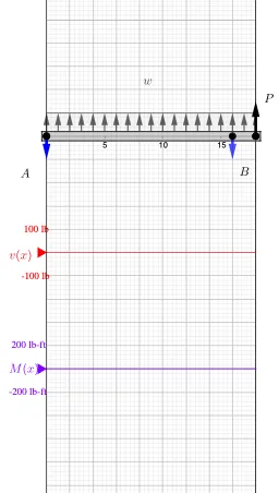
This example demonstrates the analysis of combined loads. It involves key mathematical concepts such as linear equations, trigonometric functions, and integrals. Using GeoGebra commands like Point, Vector, Polygon, etc., the load distribution can be constructed. Suitable for university engineering mechanics courses.
GeoGebra Commands & Parameters
Point(xAxis) → DPoint(xAxis) → EIf(x(D) < x(E), D, E) → startIf(start ≟ D, E, D) → endPoint(xAxis) → CPoint(xAxis) → AVector(A, Midpoint[E, D]) → r_wVector(A, C) → r_{P_1}Point(xAxis) → BSort(Unique[x({A, B, C, D, E})]) → pointsVector(A, B) → r_BPoint(x = ((-AxisStepX[])) / 4) → VMax(x({A, C, B, D, E})) → rightMin(x({A, C, B, D, E})) → leftPolygon(E + (0.2 * j), E + j, D + j, D + (0.2 * j)) → load, load_r, load_t, load_L, load_bmember((Min[x({A, C, E, D, B})], 0), (Max[x({A, C, E, D, B})], 0), (0.2 * AxisStepY[])) → beam, beam1, beam2, beam3, beam4Segment((x(A), v'(x(A))), (x(A), v'(x(A) + 0.001))) → v_ASegment((x(B), v'(x(B))), (x(B), v'(x(B) + 0.001))) → v_BPoint(x = ((-AxisStepX[])) / 4) → MSegment((x(C), v'(x(C))), (x(C), v'(x(C) + 0.001))) → v_CSegment(V', (x(V'), v'(right))) → v_rSequence(Vector[If[w > 0, Vector[E + j + (n * delta), E + (0.2 * j) + (n * delta)], Vector[E + (0.2 * j) + (n * delta), E + j + (n * delta)]]], n, 0, Length[Segment[E, D]] / abs(delta)) → distributedLoadMax(Join[{{0}, y(Sequence[Max[m, points(k), points(k + 1)], k, 1, Length[points] - 1])}]) → M_{max}Min(Join[{{0}, y(Sequence[Min[v, points(k), points(k + 1)], k, 1, Length[points] - 1])}]) → V_{min}Textfield(Scale_V) → InputBox1Textfield(Scale_M) → InputBox2Polygon((right, y(Corner[2])), (right, y(Corner[3])), Corner[3], Corner[2]) → mask, mask_l, mask_t, mask_r, mask_bSegment((0, y(V)), (right, y(V))) → VaxisSegment((0, y(M)), (right, y(M))) → MaxisMax(Join[{{0}, y(Sequence[Max[v, points(k), points(k + 1)], k, 1, Length[points] - 1])}]) → V_{max}Min(Join[{{0}, y(Sequence[Min[m, points(k), points(k + 1)], k, 1, Length[points] - 1])}]) → M_{min}If(P_C > 0, Vector[C + (1.5 * j), C], Vector[C, C + (1.5 * j)]) → p_CIf(F_B ≥ 0, Vector[B - j, B], Vector[B, B - j]) → bIf(F_A ≥ 0, Vector[A - j, A], Vector[A, A - j]) → aShuffle(Join[{{0, beamLen}, Sequence[(2 * Random[0, beamLen / 2]), n, 1, 3]}]) → temp, {2, 16, 6, 0, 16}
AI Drawing Prompt Reference
Draw a simply supported beam analysis diagram under combined loads. Place five key points on the horizontal axis, where two define the start and end of a distributed load, and the other three mark concentrated force positions. Draw vectors from the left end to each load point to represent moment arms. Within the distributed load interval, show a series of parallel arrows indicating uniform load direction with even spacing. Below the beam, plot shear force and bending moment diagrams as polyline curves, labeling their maximum and minimum values. Include two input boxes for adjusting scale factors and a masking region to hide irrelevant parts. The layout should be clear and suitable for engineering mechanics instruction.
The prompt above was compiled from the original drawing commands and is for reference only.