
Distributed Loads Analysis
Loading the math board and drawing, please wait…
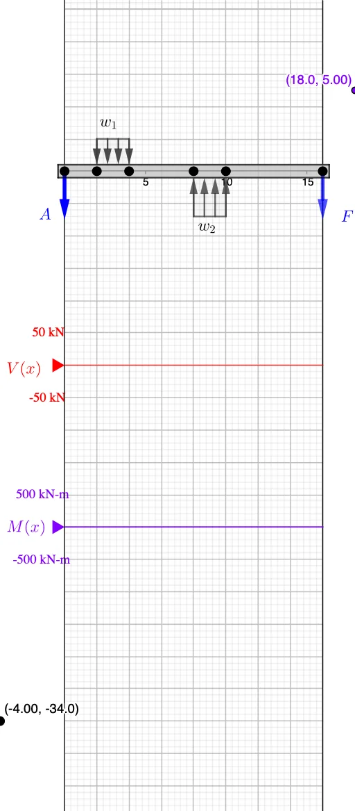
This example demonstrates the mechanical effects and moment distribution of distributed loads on a beam, involving integral calculus, derivatives, vector operations, and geometric constructions. Key GeoGebra commands and objects used include Point, Vector, If, Sort, Max, Min, member, Segment, Textfield, Polygon, Sequence for constructing load distributions, beam geometry, and force analysis. Suitable for high school students and engineering professionals studying structural mechanics and calculus applications.
GeoGebra Commands & Parameters
Point(xAxis) → CPoint(xAxis) → BPoint(xAxis) → AVector(A, Midpoint[B, C]) → r_{w_1}Point(xAxis) → EPoint(xAxis) → FVector(A, F) → r_FPoint(xAxis) → DVector(A, Midpoint[E, D]) → r_{w2}If(abs(w_1) > abs(w_2), {1.4, 1}, If[abs(w_1) < abs(w_2), {1, 1.4}, {1, 1}]) → heightIf(x(D) < x(E), D, E) → startIf(start ≟ D, E, D) → endVector(A, C) → r_{P_1}Sort(Unique[x({A, B, C, D, E, F})]) → pointsVector(A, B) → r_BMax(x({A, C, B, D, E, F})) → rightPoint(x = ((-AxisStepX[])) / 4) → VMin(x({A, C, B, D, E})) → leftIf(w_2 < 0, Polygon[E + (0.2 * j), E + (height(2) * j), D + (height(2) * j), D + (0.2 * j)], Mirror[Polygon[E + (0.2 * j), E + (height(2) * j), D + (height(2) * j), D + (0.2 * j)], xAxis]) → load_2member(A, (right, 0), (0.2 * AxisStepY[])) → beam, beam_t, beam_b, beam_r, beam_LSegment((x(A), v'(x(A))), (x(A), v'(x(A) + 0.001))) → v_ASegment((x(B), v'(x(B))), (x(B), v'(x(B) + 0.001))) → v_BPoint(x = ((-AxisStepX[])) / 4) → MSegment((x(C), v'(x(C))), (x(C), v'(x(C) + 0.001))) → v_CSegment(V', (x(V'), v'(right))) → v_rMax(Join[{{0}, y(Sequence[Max[m, points(k), points(k + 1)], k, 1, Length[points] - 1])}]) → M_{max}Min(Join[{{0}, y(Sequence[Min[v, points(k), points(k + 1)], k, 1, Length[points] - 1])}]) → V_{min}Textfield(Scale_V) → InputBox1Textfield(Scale_M) → InputBox2Polygon((right, y(Corner[2])), (right, y(Corner[3])), Corner[3], Corner[2]) → mask, mask_l, mask_t, mask_r, mask_bSegment((0, y(V)), (right, y(V))) → VaxisSegment((0, y(M)), (right, y(M))) → MaxisMax(Join[{{0}, y(Sequence[Max[v, points(k), points(k + 1)], k, 1, Length[points] - 1])}]) → V_{max}Min(Join[{{0}, y(Sequence[Min[m, points(k), points(k + 1)], k, 1, Length[points] - 1])}]) → M_{min}If(w_1 < 0, Polygon[B + (0.2 * j), B + (height(1) * j), C + (height(1) * j), C + (0.2 * j)], Mirror[Polygon[B + (0.2 * j), B + (height(1) * j), C + (height(1) * j), C + (0.2 * j)], xAxis]) → load_1If(F_A ≥ 0, Vector[A - (1.5 * j), A], Vector[A, A - (1.5 * j)]) → aIf(F_F ≥ 0, Vector[F - (1.5 * j), F], Vector[F, F - (1.5 * j)]) → fSequence(Vector[If[w_1 < 0, Vector[B + (height(1) * j) + (n * delta), B + (0.2 * j) + (n * delta)], Vector[B - (height(1) * j) + (n * delta), B - (0.2 * j) + (n * delta)]]], n, 0, Length[Segment[B, C]] / abs(delta)) → distLoad_1Sequence(Vector[If[w_2 < 0, Vector[D + (height(2) * j) + (n * delta), D + (0.2 * j) + (n * delta)], Vector[D - (height(2) * j) + (n * delta), D - (0.2 * j) + (n * delta)]]], n, 0, Length[Segment[D, E]] / abs(delta)) → distLoad_2Segment((x(F), v'(x(F))), (x(F), v'(x(F) + 0.001))) → v_F
AI Drawing Prompt Reference
Draw a cantilever beam with two distributed loads applied at both ends. Use vectors to represent the direction and magnitude of the loads. Construct the beam's geometry using points and vectors. Calculate and display the maximum and minimum bending moments and shear forces on the beam, as well as the boundary conditions. Draw the shear force and bending moment diagrams for the beam.
The prompt above was compiled from the original drawing commands and is for reference only.