
Coefficient of Variation Problems: Statistical Dispersion Visualization
Loading the math board and drawing, please wait…
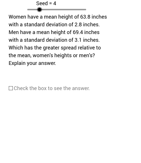
This example demonstrates the calculation and comparison of the Coefficient of Variation (CV) to measure data dispersion. Core concepts include mean, standard deviation, and CV formula. Construction uses GeoGebra commands like Element and If, with variables such as AAvg, AStDv, and ACfVr to build a dynamic model. Suitable for high school or college statistics students for interactive learning.
GeoGebra Commands & Parameters
Element(BSbSq, Seed) → BSbElement(ASbSq, Seed) → ASbElement(AAvgSq, Seed) → AAvgElement(AStDvSq, Seed) → AStDvElement(BAvgSq, Seed) → BAvgElement(BStDvSq, Seed) → BStDvIf(ACfVr > BCfVr, ASb, BSb) → WnrTxElement(ASgOPlSq, Seed) → ASgOPlElement(BSgOPlSq, Seed) → BSgOPlIf(ACfVr > BCfVr, If[ASgOPl ≟ 2, "have", "has"], If[BSgOPl ≟ 2, "have", "has"]) → VrbTxIf(ACfVr > BCfVr, If[ASgOPl ≟ 2, "their", "its"], If[BSgOPl ≟ 2, "their", "its"]) → PsTx