
Cobweb Plot of a Linear Function
Loading the math board and drawing, please wait…
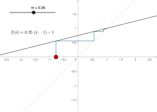
This example demonstrates the cobweb plot of a linear function, illustrating the dynamic relationship between iterations and initial values. Key math concepts include function iteration, linear function properties, and coordinate geometry. It utilizes GeoGebra commands and objects like Intersect, Point, Iteration, Sequence, and Segment as outlined in the construction summary. Suitable for high school mathematics education to visually understand function iteration and dynamic changes.
GeoGebra Commands & Parameters
Intersect(f, g, (1, 1)) → A_1Intersect(f, g, (1, 1)) → BPoint(xAxis) → AIteration(f, x(A_1), n) → aSequence(Iteration[f, x(A), i], i, 1, n) → L_1Sequence(Segment[(L_1(i), L_1(i)), (L_1(i), L_1(i + 1))], i, 1, Length[L_1] - 1) → L_2Sequence(Segment[(L_1(i), L_1(i + 1)), (L_1(i + 1), L_1(i + 1))], i, 1, Length[L_1] - 1) → L_3Segment(A, (x(A), f(x(A)))) → hSegment((x(A), f(x(A))), (f(x(A)), f(x(A)))) → i
AI Drawing Prompt Reference
Draw a cobweb plot for a linear function, showing the dynamic relationship between iterations and initial values. Start by plotting the coordinate axes and the linear function. Then, from the point (1,1), iteratively generate a sequence of points by intersecting the function with the axes. Connect these points with line segments to form a cobweb pattern. Finally, connect the initial point to its function value and the function value to itself to complete the plot.
The prompt above was compiled from the original drawing commands and is for reference only.