
Cobweb Diagram Visualization
Loading the math board and drawing, please wait…
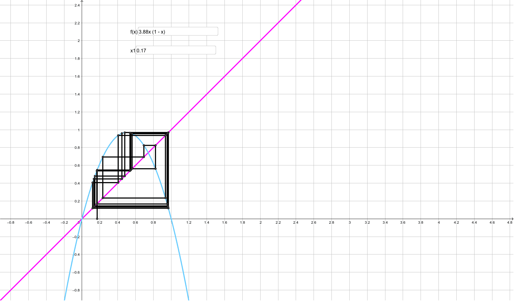
This example demonstrates cobweb diagrams, visualizing the dynamic behavior of iterative function sequences. Key math concepts include function iteration, difference equations, slope analysis, and angle relationships. Construction highlights involve using GeoGebra's Segment and Textfield commands to plot function graphs, points, and dynamic connections. Suitable for high school and above learners studying discrete dynamical systems and function iteration properties.
GeoGebra Commands & Parameters
Segment(U, B) → hSegment(B, V) → iSegment(V, C) → jSegment(C, W) → kSegment(W, D) → lSegment(D, Z) → mSegment(Z, E) → nSegment(E, A_1) → pSegment(A_1, F) → qSegment(B_1, F) → rSegment(B_1, G) → sSegment(G, C_1) → tSegment(C_1, H) → aSegment(H, D_1) → bSegment(D_1, I) → cSegment(I, E_1) → dSegment(E_1, J) → eSegment(J, F_1) → f_1Segment(F_1, K) → g_1Segment(K, G_1) → h_1Segment(G_1, L) → i_1Segment(L, H_1) → j_1Segment(H_1, M) → k_1Segment(M, I_1) → l_1Segment(I_1, N) → m_1Segment(N, J_1) → n_1Segment(J_1, O) → p_1Segment(O, K_1) → q_1Segment(K_1, P) → r_1Segment(P, L_1) → s_1Segment(L_1, Q) → t_1Segment(Q, M_1) → a_1Segment(M_1, R) → b_1Segment(R, N_1) → c_1Segment(N_1, S) → d_1Segment(S, O_1) → e_1Segment(O_1, T) → f_2Textfield(g) → InputBox1Textfield(B1) → InputBox2