
Class Size and Standardized Test Performance: Linear Fit and Correlation Analysi
Loading the math board and drawing, please wait…
In collections
CCSS IP Math I Unit 4 Lesson 3
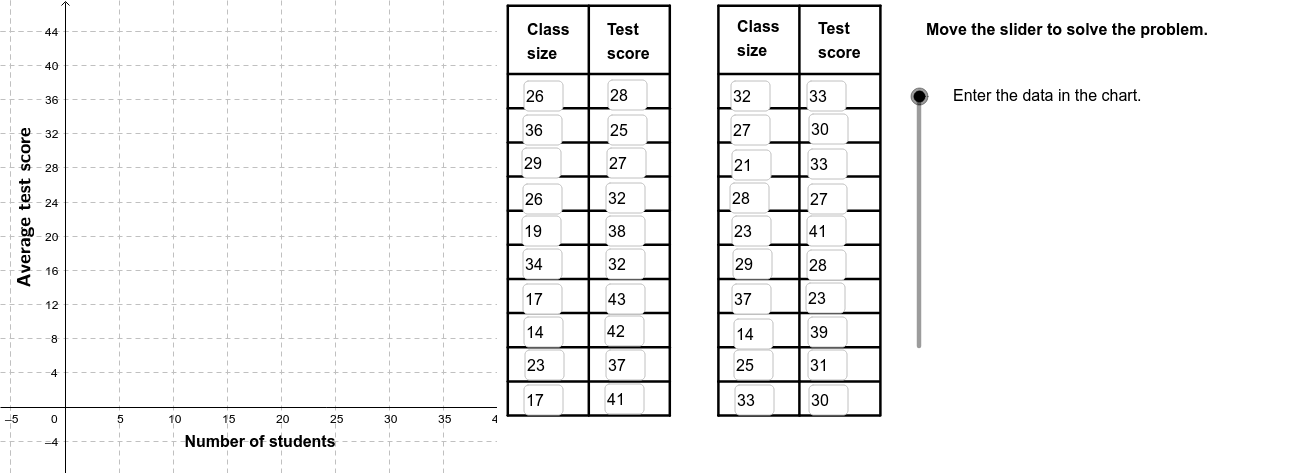
This example demonstrates the possible linear relationship between class size and student performance on standardized tests, using a scatter plot with a fitted regression line to visualize the correlation between two variables. Core mathematical concepts include Pearson’s product-moment correlation coefficient (PMCC), least-squares linear fitting (FitLineY), conditional logic (If), and coordinate representation of data points. Construction-wise, the GeoGebra commands FitLineY, PMCC, Textfield, If, Polygon, Sequence, Segment, and RotateText are employed together with objects A1 through B19 to build the scatter plot, regression line, dynamic text annotations, conditional displays, and auxiliary geometric elements. It is suitable for high school statistics and probability courses, as well as introductory data analysis and correlation visualization exercises.
GeoGebra Commands & Parameters
FitLineY(PointList1) → LineFitPMCC(PointList1) → CorCoeffTextfield(A2) → InA2Textfield(A3) → InA3Textfield(A4) → InA4Textfield(A5) → InA5Textfield(A6) → InA6Textfield(A7) → InA7Textfield(A8) → InA8Textfield(A9) → InA9Textfield(A10) → InA10Textfield(A11) → InA11Textfield(A12) → InA12Textfield(A13) → InA13Textfield(A14) → InA14Textfield(A15) → InA15Textfield(A16) → InA16Textfield(A17) → InA17Textfield(A18) → InA18Textfield(A19) → InA19Textfield(A20) → InA20Textfield(A21) → InA21Textfield(B2) → InB2Textfield(B3) → InB3Textfield(B4) → InB4Textfield(B5) → InB5Textfield(B6) → InB6Textfield(B7) → InB7Textfield(B8) → InB8Textfield(B9) → InB9Textfield(B10) → InB10Textfield(B11) → InB11Textfield(B12) → InB12Textfield(B13) → InB13Textfield(B14) → InB14Textfield(B15) → InB15Textfield(B16) → InB16Textfield(B17) → InB17Textfield(B18) → InB18Textfield(B19) → InB19Textfield(B20) → InB20Textfield(B21) → InB21If(CorVisible, "Hide Correlation Coefficient", "Show Correlation Coefficient") → CorButtonIf(LineVisible, "Hide Best Fit Line", "Show Best Fit Line") → LineButtonPolygon((40, y(Corner[1])), Corner[2], Corner[3], (40, y(Corner[4]))) → poly1, a, b, c, dSequence(Segment[(41, -1 + (4 * i)), (56, -1 + (4 * i))], i, 0, 10) → Linesh1Sequence(Segment[(41 + (7.5 * i), -1), (41 + (7.5 * i), 47)], i, 0, 2) → Linesv1Sequence(Segment[(60.5 + (7.5 * i), -1), (60.5 + (7.5 * i), 47)], i, 0, 2) → Linesv2Sequence(Segment[(60.5, -1 + (4 * i)), (75.4, -1 + (4 * i))], i, 0, 10) → Linesh2Segment((41, 47), (56, 47)) → top1Segment((60.5, 47), (75.5, 47)) → top2RotateText("Average test score", 90*°) → SideLegend
AI Drawing Prompt Reference
Create a scatter plot showing the relationship between class size and standardized test scores with about twenty data points, a least‑squares regression line, a text label displaying the Pearson correlation coefficient, and two toggle buttons to show or hide the correlation value and the fitted line; on the right side add a rectangular panel containing horizontal and vertical grid lines.
The prompt above was compiled from the original drawing commands and is for reference only.