
Center & Spread Exploration: Mean, Median, Quartiles, and Standard Deviation
Loading the math board and drawing, please wait…
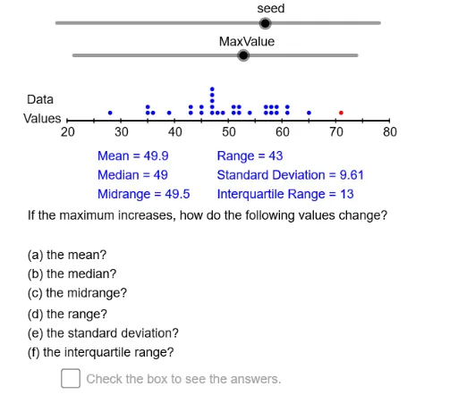
This interactive GeoGebra example dynamically visualizes how measures of central tendency (mean, median) and spread (range, interquartile range, standard deviation) respond to changes in a dataset. It demonstrates the construction of statistical summaries using a dot plot or similar representation, with sliders to adjust data values. Core mathematical concepts include descriptive statistics: mean, median, quartiles (Q1, Q3), range, IQR, and standard deviation, as well as data sorting and frequency distribution. The construction uses GeoGebra commands such as Sequence, Sort, CountIf to generate and organize data; Min, Max, Append, Union to compute extremes and merge lists; mean, Median, Q1, Q3, stdev for statistical calculations; and Segment, If, Slider for dynamic graphics and user interaction. This resource is ideal for middle school to high school statistics lessons, helping students grasp how different statistics summarize data distribution and how center and spread complement each other. It serves both as a classroom demonstration tool and for independent student exploration.
GeoGebra Commands & Parameters
Mod(10 + (37 * seed), 80) → Nmbr1Sequence(RandomPoisson[seed], k, 1, size) → Dt1Max(Dt1) → DtMx1Min(Dt1) → DtMn1Sequence(k, k, DtMn1 - 10, DtMx1 + 10) → DmnSequence(k, k, DtMn1, DtMx1) → DmnMdAppend(Append[Dt1, DtMn2], DtMx2) → Dt2Union(Intersection[Dt1, DmnMd], {DtMn2, DtMx2}) → DtExtSort(Intersection[Dmn, DtExt]) → RngCountIf(x < DtMx2 + 1, Rng) → RngCntSequence(CountIf[x ≟ Element[Rng, k], Dt1], k, 1, RngCnt) → FrqSqSegment(LE, RE) → haxisSequence(Segment[((k * AxScl), -0.01), ((k * AxScl), 0.01)], k, 0, AxRE - AxLE, 5) → HTcsSequence(Text[k, (adp(k) - 1, -0.08)], k, AxLE, AxRE, 10) → HAxLblIf(MinOrMax ≟ 1, "minimum", "maximum") → MnOrMxIf(DownOrUp ≟ 1, "decreases", "increases") → DnOrUpmean(Dt2) → DtAvgMedian(Dt2) → DtQ2Q1(Dt2) → DtQ1Q3(Dt2) → DtQ3stdev(Dt2) → DtSDIf(DownOrUp ≟ 1, "increases", "decreases") → UpOrDnIf(MinOrMax ≟ 1, If[DownOrUp ≟ 1, "increases", "decreases"], If[DownOrUp ≟ 1, "decreases", "increases"]) → SpChSequence(Sequence[(adp(Element[Rng, k]), 0.01 + (0.03 * j)), j, 1, Element[FrqSq, k]], k, 1, RngCnt) → Dts1If(DtMn2 ≟ DtMn1, (adp(DtMn2), 0.04 + (0.03 * Element[FrqSq, 1])), (adp(DtMn2), 0.04)) → MnDtMnIf(DtMx2 ≟ DtMx1, (adp(DtMx2), 0.04 + (0.03 * Element[FrqSq, RngCnt])), (adp(DtMx2), 0.04)) → MxDtMxIf(DtMn2 ≟ DtMn1, (adp(DtMn2), 0.04 + (0.03 * Element[FrqSq, 1])), (adp(DtMn2), 0.04)) → MnDtMxIf(DtMx2 ≟ DtMx1, (adp(DtMx2), 0.04 + (0.03 * Element[FrqSq, RngCnt])), (adp(DtMx2), 0.04)) → MxDtMn
AI Drawing Prompt Reference
Create an interactive statistical chart showing a dot plot of a random dataset along a horizontal axis, with dots stacked vertically to represent frequency. Display dynamic text labels for the mean, median, first and third quartiles, range, interquartile range, and standard deviation. Include sliders to adjust data values, and markers to highlight the minimum and maximum points. Add a baseline axis with tick marks and numeric labels. The chart should update in real time as data changes, helping users explore how measures of center and spread respond to modifications.
The prompt above was compiled from the original drawing commands and is for reference only.