
Biscribed Truncated Icosidodecahedron n=120, Polyhedra with Extreme Vertex Distr
Loading the math board and drawing, please wait…
In collections
₈Polyhedra with extreme distribution of equivalent vertices
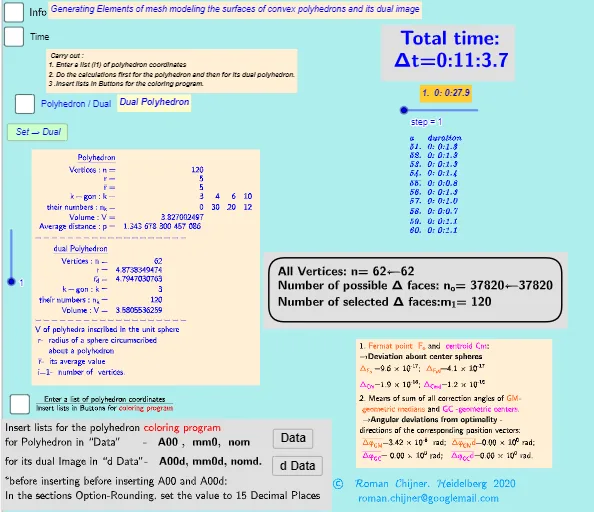
This example demonstrates the geometric construction of a Biscribed Truncated Icosidodecahedron n=120, highlighting the extreme distribution of equivalent vertices in polyhedra. Core mathematical concepts include polyhedral construction, vertex distribution, and geometric optimization. The construction utilizes GeoGebra commands and objects such as Text, Sum, If, Length, Sequence, Div, Element, TableText, IndexOf, First, and Max to achieve complex parameterized modeling. Suitable for high school students and geometry enthusiasts, this example aids in understanding polyhedral geometry and optimization problems.
GeoGebra Commands & Parameters
Text("" + p) → txt_pSum(Flatten[Sequence[Append[Sequence[Element[txt_p, i], i, m01(k), m02(k)], " "], k, 1, 5]]) → txtUm1If(bu0, A00, A00d) → A00_0Length(A00_0) → nLength(l2) → läl2Sequence(sgn(Determinant[{Element[A00_0, i1] - Element[A00_0, j], Element[A00_0, i2] - Element[A00_0, j], Element[A00_0, i3] - Element[A00_0, j]}]), j, 1, n) → l01Length(A00d) → zzzSum(Zip[(T * F), T, SysTimeAkt1, F, {1, 1000, 60000, 3600000, 86400000}]) → TimeAbs1Sum(Zip[(T * F), T, SysTimeAkt2, F, {1, 1000, 60000, 3600000, 86400000}]) → TimeAbs2Div(TimeRelab, 3600) → HDiv(TimeRelab - (H * 3600), 60) → MElement(ZwZeit, step) → text10TableText({Append["a duration", Last[ZwZeit, Min[10, Length[ZwZeit]]]]}, "v") → text2cLength(A00) → lm1If(Length[Unique[l01 \ {0}]] ≟ 1, 7, -7) → a7Sum(Zip[(T * F), T, SysTimeAkt0, F, {1, 1000, 60000, 3600000, 86400000}]) → TimeAbs0Div(TimeRelab0, 3600) → H0Div(TimeRelab0 - (H0 * 3600), 60) → M0Text("" + (TimeRelab0 - (H0 * 3600) - (M0 * 60))) → S0aText("" + (TimeRelab - (H * 3600) - (M * 60))) → SIndexOf(".", S) → indexIndexOf(".", S0a) → indexaFirst(S, index + 1) → txtSFirst(S0a, indexa + 1) → txtS0aIf(bu0, " ", "d") → txtbuoMax(Length[A00], Length[A00d]) → maxläElement(A00, 24) → m11TableText({{"\underline{Polyhedron}"}, Append["Vertices: n=", {Length[A00]}], Append["r=", {r}], Append["\bar{r}=", {r_m}], Append["k-gon : k=", mm5a], Append["their\; numbers: n_k=", mm7a], Append["Volume: V=", {Vol_r}], Append["Average\; distance: p=", {txtUm1}]}, "hr ") → text7TableText({{"\underline{dual\;Polyhedron}"}, Append["Vertices: n=", {Length[A00d]}], Append["r=", {r_d}], Append[" \bar{r_d}= ", {r_md}], Append["k-gon : k=", mm5ad], Append["their\; numbers: n_k=", mm7ad], Append["Volume: V=", {Vold_r}]}, "hr ") → text20
AI Drawing Prompt Reference
Construct a biscribed truncated icosidodecahedron with parameterized vertex set using n=120, and visualize both the polyhedron and its dual. First include textual annotations for the parameters and computed statistics. Then build the vertex set by evaluating a determinant/sign condition from indexed triples of vertex coordinates, using the resulting indices to generate the required vertices and ensure the desired extreme-equivalent-vertex distribution. After the polyhedra are formed, add a summary in the figure for each of the polyhedron and the dual, listing their vertex counts, the values r and r̄, the k-gon parameter k with the associated vertex numbers n_k, and the computed volume V and average distance p.
The prompt above was compiled from the original drawing commands and is for reference only.