
Binomial Distribution by Chris Mizell
Loading the math board and drawing, please wait…
In collections
Probabilty
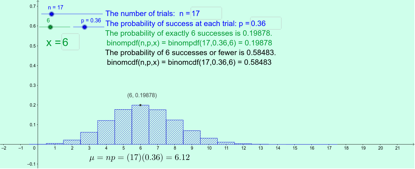
This example visualizes the shape of the binomial distribution for different numbers of trials and success probabilities. It involves key concepts such as the number of trials and success probability. Using GeoGebra commands like Sequence and BinomialDist, users can dynamically adjust parameters to observe changes in the distribution. Suitable for high school mathematics education and learning probability statistics.
GeoGebra Commands & Parameters
Sequence(Binomial[n, k] * p^(k) * (1 - p)^(n - k), k, 0, n) → list1Sequence(Sum[list1, k], k, 1, n + 1) → list2BinomialDist(n, p) → aTextfield(p) → inputBox1Textfield(n) → inputBox2Element(list1, S + 1) → bElement(list2, S + 1) → cTextfield(S) → inputBox3Sequence((i, Element[list1, i + 1]), i, 0, n) → list3
AI Drawing Prompt Reference
Draw a binomial distribution graph by changing the number of trials n and success probability p to observe changes in the distribution shape. First, input the values of n and p, then generate the binomial probability mass function based on n and p, calculate the cumulative distribution function, and finally plot the binomial probability mass function graph.
The prompt above was compiled from the original drawing commands and is for reference only.